23 · When You Can’t Flip the Coin

On Monday 26 October, Dana had the agenda for Friday’s board meeting on her desk. One line was circled in red.

“The twelve percent is closed,” she said. “Thank you. Now I have a smaller question, and it is harder, because this time I can’t blame the dashboard.”

She turned the page around. The circled line said: Riverside fee: what did it cost?

“Riverside’s city council passed a rule about courier costs. To pay for it, we added $0.99 to the delivery fee of every consumer order in Riverside, from Monday 5 October. The board will ask what it cost us. Priya would say: run an A/B test. We can’t. It is a city law. Everyone in Riverside pays it, and nobody outside Riverside does.”

“So nobody can flip a coin,” Mia said.

“Nobody can flip a coin.”

The fee was easy to find in the data. In Riverside, the average delivery fee on consumer orders went from $2.81 before 5 October to $3.81 after it. In the other cities, it stayed at about $2.24.

Back at her desk, Mia wrote three lines in her notebook:

Three weeks before: 14 Sep–4 Oct. Three weeks after: 5–25 Oct. Three other cities, with no fee.

Then she made the first comparison anyone would make. Riverside had 20,241 completed orders in the three weeks before the fee and 19,925 in the three weeks after (final statuses, see Chapter 1). That is a change of −1.6%.

Theo read it over her shoulder. “Down 1.6%. Small. Dana will like that.”

“Dana will like it,” Mia said. “That is why I don’t trust it yet.”

ImportantThe big idea

When you cannot flip a coin, compare the group that changed with a group that moved the same way before the change, and measure how far the two moved apart after it.

Picture the two rows of tea bushes at the top of this chapter. They grow in the same soil and weather, at the same pace. Halfway along, the lower row passes through a gate, and after it, its bushes are a little shorter. You can never see how tall they would have grown without the gate, but the upper row is your best guess. Riverside is the lower row, the other three cities are the upper row, and the gate is 5 October.

Why a coin is so good

In an A/B test (Chapter 20), a coin decides who sees the change. The coin does not care who drinks a lot of tea or who orders more when it rains. So the two groups end up alike in everything, measured or not. If they differ afterwards, the cause is the change or luck, and the p-value (Chapter 18) tells you how much luck could do.

Working out what caused what is called causal inference. An A/B test is its easy case. Most of the time you have observational data: records of a world you watched but did not control.

The Riverside fee is a better case than most. It is a natural experiment: a change that the world, not you, gave to some people and not to others, for a reason that has nothing to do with the result you measure. The council chose Riverside because it governs Riverside, not because its customers were about to order less tea. The problem is that a city law is one flip of a coin, not thousands: one city, one date, and everything else that happened in those weeks came along with it.

What else changed on 5 October?

Mia’s −1.6% compares Riverside with its own past. It quietly assumes that, without the fee, the three weeks after would have looked like the three weeks before.

What would have happened without the change is called the counterfactual. You can never observe it: there is no second Riverside without the fee. Every method in this chapter is a way to make a good guess at it.

Riverside’s own past is a weak guess here, because the world did not stand still. Steep grows a little each week (Chapter 16), and the weather moved too. Riverside had 5 rainy days in the three weeks before the fee and 8 in the three weeks after. Rain brings orders: on a rainy day, more people open the app (Chapter 16).

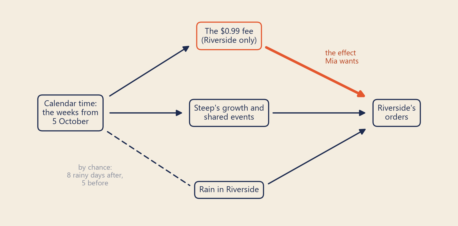
Mia drew this as a causal diagram: a picture of what pushes on what. Each box is something that can change. Each arrow means “this pushes on that”.

fig, ax = bk.figure(8, 3.9)
ax.set_xlim(0, 10)
ax.set_ylim(0, 6)
ax.axis("off")
boxes = {
    "time": (1.45, 3.0, f"Calendar time:\nthe weeks from\n{day_month(START)}"),
    "fee": (5.0, 5.15, "The $0.99 fee\n(Riverside only)"),
    "shared": (5.0, 3.0, "Steep's growth and\nshared events"),
    "rain": (5.0, 0.85, "Rain in Riverside"),
    "orders": (8.75, 3.0, "Riverside's\norders"),
}
for key, (x, y, label) in boxes.items():
    edge = bk.TOMATO if key == "fee" else bk.INK
    ax.text(x, y, label, ha="center", va="center", fontsize=10.5, color=bk.INK,
            bbox=dict(boxstyle="round,pad=0.55", fc=bk.PAPER, ec=edge, lw=1.4))


def arrow(start, end, color=bk.INK, lw=1.6, style="-|>", ls="-"):
    ax.annotate("", xy=end, xytext=start,
                arrowprops=dict(arrowstyle=style, color=color, lw=lw, ls=ls, mutation_scale=16))


arrow((2.3, 3.45), (4.15, 4.9))
arrow((2.3, 3.0), (4.0, 3.0))
arrow((5.8, 4.85), (8.1, 3.42), color=bk.TOMATO, lw=3.2)
arrow((5.95, 3.0), (8.1, 3.0))
arrow((5.85, 1.0), (8.1, 2.58))
arrow((2.25, 2.5), (4.15, 0.95), style="-", ls=(0, (4, 3)))
ax.text(2.0, 1.25, f"by chance:\n{riv_rain_post} rainy days after,\n{riv_rain_pre} before",
        ha="center", va="center", fontsize=9, color=bk.MUTED)
ax.text(7.15, 4.55, "the effect\nMia wants", ha="left", va="center", fontsize=9.5,
        color=bk.TOMATO_TEXT)
plt.show()

Figure 1: Mia’s causal diagram. Boxes are things that can change; solid arrows mean “pushes on”. The dashed line is not a cause: in these weeks, extra rain and the fee arrived together by chance.

The arrow Mia wants is the tomato one, from the fee to Riverside’s orders. But calendar time also carries Steep’s growth and anything else every city shared in those weeks, and by chance it brought Riverside more rain. A before/after comparison adds up all the arrows into Riverside’s orders and calls the total “the fee”.

Chapter 4 called this kind of thing a confounder: a third thing that affects both the groups you compare and the result you measure. Here the two groups are days: the days before 5 October and the days after. Calendar time decides which group a day is in, and so whether Riverside has the fee that day. It also moves orders in other ways, through growth and shared events. When a confounder is at work, a plain comparison mixes its effect with the effect you want. That mixing is called confounding.

Borrow a twin: difference-in-differences

Mia needed something that went through the same weeks as Riverside, with the same growth, app, menu and prices, but with no fee. Steep has three: Harbor, Northgate and Oldtown.

Completed orders	Before (14 Sep–4 Oct)	After (5–25 Oct)	Change
Riverside (the fee)	20,241	19,925	−1.6%
Other three cities (no fee)	115,210	117,446	+1.9%
Riverside compared with the others			−3.4%

The other cities grew 1.9%. If Riverside had grown like them, its 20,241 orders would have become about 20,634. It had 19,925: about 709 fewer, or 3.4% below what the other cities predict.

This calculation is called difference-in-differences, or DiD. Take the change in the group that got the treatment. Take away the change in a comparison group that did not get it. What is left is the part of the change that the comparison group cannot explain. In a famous study, two economists compared fast-food restaurants in New Jersey, where the minimum wage rose in 1992, with restaurants in nearby Pennsylvania, where it did not (Card and Krueger, 1994).

Mia compared changes in percent, not in orders. Harbor has about 2.7 times as many orders as Riverside, so if rain lifts every city by 2%, Harbor gains far more orders. “Moving the same way” means moving by the same percent.

Parallel trends: the assumption you can partly check

DiD rests on one assumption. Without the fee, Riverside’s orders would have moved in parallel with the other cities’: the same percent ups and downs. This is called parallel trends.

You cannot check it after 5 October: that is the world nobody can see. But you can check it before. If Riverside and the others moved together for months, it is a fair guess that they would have kept moving together for three more weeks.

weekly = (panel.assign(group=np.where(panel.city == CITY, "riverside", "others"),
                       week=panel.day - pd.to_timedelta(panel.day.dt.weekday, unit="D"))
          .groupby(["week", "group"]).orders.sum().unstack("group"))
index = 100 * weekly / weekly.loc[T(PRE[0]):T(PRE[1])].mean()
mid = index.index + pd.Timedelta(days=3)

fig, ax = bk.figure(8, 4.0)
ax.axvspan(T(PRE[0]), T(PRE[1]) + DAY, color=bk.TEAL, alpha=0.10, lw=0)
ax.axvspan(START, T(POST[1]) + DAY, color=bk.TOMATO, alpha=0.10, lw=0)
ax.axvline(START, color=bk.INK, lw=1, ls="--")
ax.plot(mid, index.others, color=bk.TEAL, lw=2.2, marker="o", ms=3.5)
ax.plot(mid, index.riverside, color=bk.TOMATO, lw=2.2, marker="o", ms=3.5)
top = index.max().max()
ax.text(START - 2 * DAY, top + 1.2, f"fee starts {day_month(START, short=True)}",
        ha="right", fontsize=9.5)
ax.text(mid[0], top + 2.2, "Other three cities", color=bk.TEAL_TEXT, fontsize=10)
ax.text(mid[0], top + 1.0, "Riverside", color=bk.TOMATO_TEXT, fontsize=10)
ax.set_ylim(index.min().min() - 1.5, top + 3.4)
ax.set_ylabel("Weekly orders\n(14 Sep–4 Oct = 100)")
ax.xaxis.set_major_locator(mdates.MonthLocator())
ax.xaxis.set_major_formatter(mdates.DateFormatter("%b"))
ax.set_title("All summer, Riverside moved with the other cities. After the fee, it fell behind.")
plt.show()

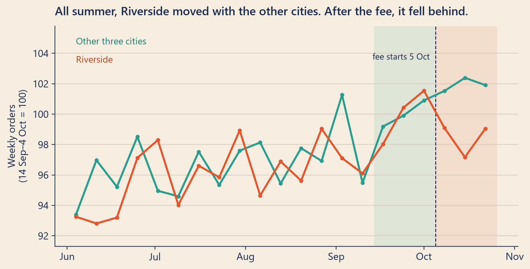
Figure 2: Weekly completed orders, each line divided by its own weekly average over the three weeks before the fee (14 September – 4 October = 100). The shaded bands are the two windows Mia compared.

From June to early October, the two lines move together. Both wobble with the rain, which falls on each city separately, but around the same path. After 5 October, Riverside’s line sits below the other line for three weeks in a row.

Parallel lines before a change do not prove that they would have stayed parallel after it. Something else could have hit Riverside alone on the same day, such as a new competitor, and DiD would blame the fee for that too. But lines that drift apart before the change are a clear warning, and these lines do not drift.

Rain: an unlucky coincidence

The table treats every day alike. But rain did not fall evenly. Riverside had 5 rainy days before the fee and 8 after it. The other three cities had 16 rainy city-days (one city on one day) before and 18 after, out of 63 each time: a much smaller change. Rain raises orders, so the extra rain lifted Riverside’s after-window and hid part of what the fee cost. Rain did not cause the fee. By chance, extra rain fell in the same weeks, so rain got mixed into the comparison.

The repair is to measure the rain and take it out. Like Chapter 16’s recipe for a normal day, Mia’s recipe for each city’s daily orders has four parts:

• a level for each city (Harbor is big, Riverside is small);
• a level for each day, shared by all the cities (weekdays, growth, anything that hit every city that day);
• a lift for a rainy day in a city;
• the fee: a change that switches on for Riverside only, from 5 October.

The computer finds the numbers that make the recipe fit the real days best. This is a regression. The shared day levels do the job of the comparison cities. Putting a variable such as rain into the recipe is called controlling for it: the fee is then measured as if the rain had been the same.

The recipe	Fee’s effect on Riverside’s orders	95% interval
City and day levels, no rain	−3.3%	−6.2% to −0.4%
City and day levels, plus rain	−4.5%	−6.4% to −2.6%

A rainy day lifts a city’s orders by about 12%. With rain in, the estimate grew, because rain had been hiding part of the drop. The interval got narrower, because rain explains much of the daily noise. The p-value is below 0.001, but read it as a rough guide (Under the hood says why). The fake dates in the next section are a sturdier check.

In orders, −4.5% means that Riverside placed about 943 fewer orders in three weeks than it would have without the fee (range 532 to 1,362).

NoteUnder the hood

For city \(c\) on day \(t\), the recipe is

\[\log(\text{orders}_{ct}) = \alpha_c + \lambda_t + \gamma \cdot \text{rain}_{ct} + \delta \cdot D_{ct} + \varepsilon_{ct},\]

where \(\alpha_c\) is a city level, \(\lambda_t\) a day level shared by all cities, \(\text{rain}_{ct}\) is 1 on a rainy day, and \(D_{ct}\) is 1 for Riverside from 5 October and 0 otherwise. On the log scale, a difference is a percent change, which is why “parallel” means “the same percent”. The fee’s effect is \(e^{\delta} - 1\) = −4.5%; the rain lift is \(e^{\gamma} - 1\) = +11.7%. The regression uses 168 city-days.

Without rain, \(\hat\delta\) is Riverside’s change in average log orders minus the other cities’ average change: −3.3%. The table’s −3.4% weights the other cities by size instead.

The standard errors are robust (HC1): they allow some days to be noisier than others, but assume that one day’s noise is unrelated to the next day’s. If that is wrong, the intervals are too narrow (Bertrand, Duflo and Mullainathan, 2004). The usual fix, clustering by city, cannot work with only one treated city, however many comparison cities you add (Conley and Taber, 2011).

The fake dates below need no such assumption. Their estimates have a standard deviation of 1.01 points, about the real estimate’s standard error (1.01), so the intervals look about right. The real estimate is the most extreme of 14 dates, which on rank alone gives p = 1/14 ≈ 0.07, the smallest possible. Its distance says more: about 4.7 standard deviations below the fake estimates’ average.

The playground uses a shortcut. Every city has every day, so you can remove the city and day levels by subtracting each city’s average and each day’s average and adding back the overall average. A regression of what is left on rain and \(D\) gives the same \(\hat\delta\) (the Frisch–Waugh–Lovell theorem); this chapter checks that they agree.

A fake gate: the placebo test

Mia wanted one more check before she believed −4.5%. What would the method say about a date when nothing happened?

She pretended that the fee had started on Monday 21 September, and ran the same recipe on the two weeks before it (7–20 Sep) and the two weeks after (21 Sep–4 Oct). Why two weeks, not three? The fake after-window must end before the real fee, and only two weeks fit. This is a placebo test: you run your method where you know the true effect is zero. (In medicine, a placebo is a sugar pill that should do nothing.)

The fake fee “changed” Riverside’s orders by −1.1%, with an interval from −3.5% to +1.3% and p = 0.357. No sign of an effect, as it should be.

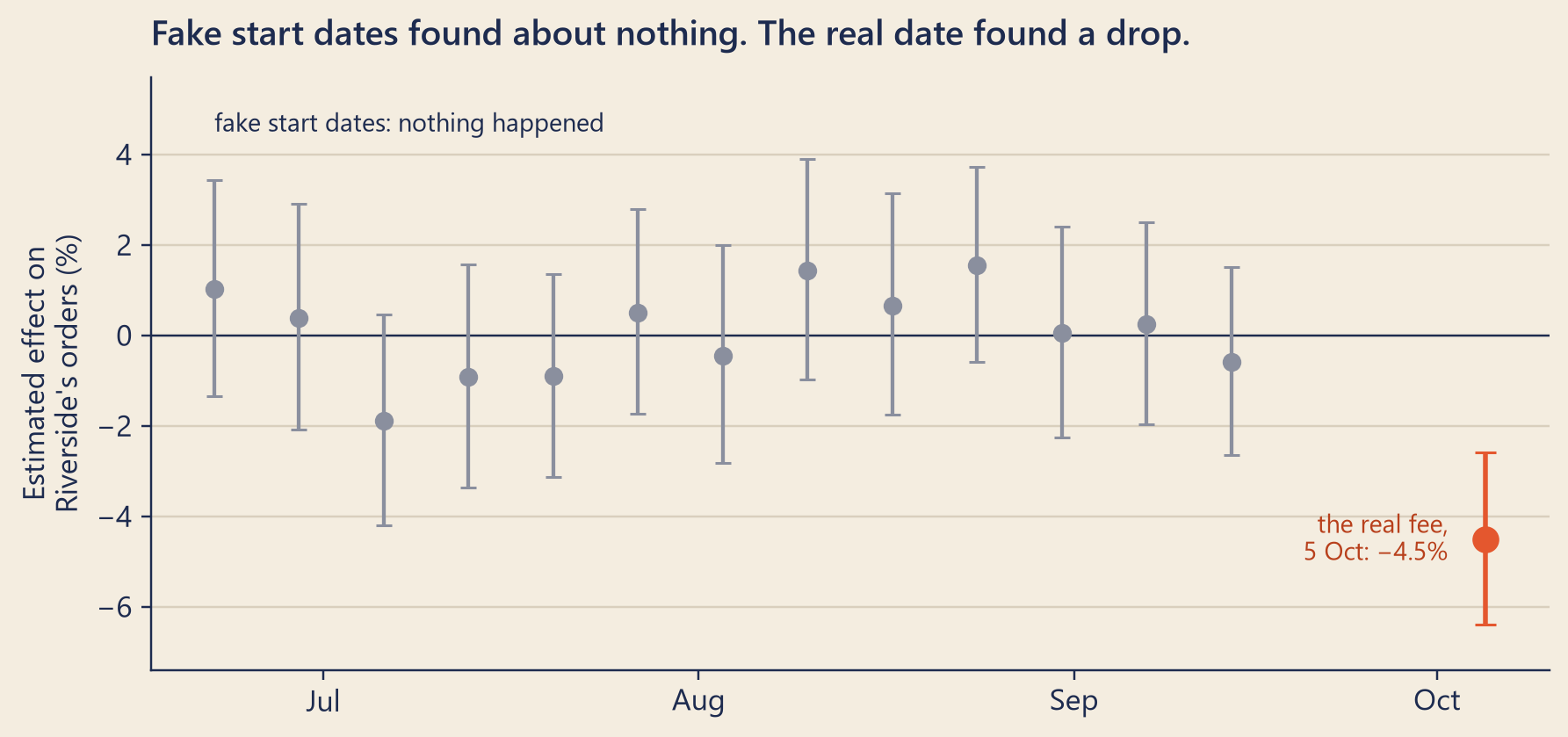
One fake date could pass by luck. So Mia tried every Monday of the summer as a fake start, each with three weeks on each side, the same windows as the real analysis. The last Monday with room for three weeks before the real fee is 14 September.

fig, ax = bk.figure(8, 3.7)
ax.axhline(0, color=bk.INK, lw=0.8)
ax.errorbar(fakes.day, 100 * fakes.effect,
            yerr=[100 * (fakes.effect - fakes.lo), 100 * (fakes.hi - fakes.effect)],
            fmt="o", color=bk.MUTED, ecolor=bk.MUTED, ms=6, capsize=3, lw=1.4)
ax.errorbar([START], [100 * est.effect],
            yerr=[[100 * (est.effect - est.ci_low)], [100 * (est.ci_high - est.effect)]],
            fmt="o", color=bk.TOMATO, ecolor=bk.TOMATO, ms=9, capsize=4, lw=1.8)
ax.annotate(f"the real fee,\n{day_month(START, short=True)}: {pct(est.effect)}",
            (START, 100 * est.effect), xytext=(-14, 0), textcoords="offset points",
            ha="right", va="center", fontsize=9.5, color=bk.TOMATO_TEXT)
ax.text(fakes.day.iloc[0], 100 * fakes.hi.max() + 0.6, "fake start dates: nothing happened",
        fontsize=9.5, color=bk.INK)
ax.set_ylabel("Estimated effect on\nRiverside's orders (%)")
ax.set_ylim(100 * est.ci_low - 1, 100 * fakes.hi.max() + 1.8)
ax.xaxis.set_major_locator(mdates.MonthLocator())
ax.xaxis.set_major_formatter(mdates.DateFormatter("%b"))
ax.set_title("Fake start dates found about nothing. The real date found a drop.")
plt.show()

Figure 3: The same recipe (city, day and rain) run with fake start dates, three weeks before and three weeks after each, all before the real fee. Bars show 95% intervals.

All 13 fake estimates lie between −1.9% and +1.5%, and every interval includes zero. The method found nothing on 13 dates when nothing happened, and a clear drop, −4.5%, on 5 October.

Why the first answer misled

Comparison	Riverside’s change	What it still contains
Riverside after vs before	−1.6%	Steep’s growth, shared events, Riverside’s extra rain
DiD against the other cities	−3.3%	Riverside’s extra rain
DiD with rain in the recipe	−4.5%	nothing we know of

The first answer had the right sign but about a third of the size: it understated the drop by 3.0 points. Two things pushed it toward zero. The other cities grew 1.9% over the same weeks, and Riverside would likely have grown with them. And Riverside had extra rain.

Try it: build your own DiD

This playground runs Mia’s recipe on the real daily orders of the four cities. Pick the comparison cities, the windows, rain on or off, and the start date. An earlier Monday makes it a placebo test, and the after-window then stops on 4 October, so the real fee never leaks in.

viewof didCities = Inputs.checkbox(
  new Map(ch23.others.map((c) => [c[0].toUpperCase() + c.slice(1), c])),
  {label: "Comparison cities", value: ch23.others}
)
viewof didStart = Inputs.select(didMondays, {label: "Change starts on", value: ch23.realStart})
viewof didBefore = Inputs.range([1, 6], {value: 3, step: 1, label: "Weeks before"})
viewof didAfter = Inputs.range([1, 3], {value: 3, step: 1, label: "Weeks after"})
viewof didRain = Inputs.toggle({label: "Control for rain", value: true})

didReadout = {
  if (!didResult) return html`<p><strong>Pick at least one comparison city.</strong></p>`;
  const r = didResult, w = didWindows;
  const per = (x) => Math.round(x).toLocaleString("en-US");
  const interval = `${signedPct(r.lo)} to ${signedPct(r.hi)}`;
  const covers = r.lo < 0 && r.hi > 0;
  const verdict = w.isPlacebo
    ? (covers
      ? "This is a placebo: nothing happened on that date. The interval includes 0, so the method sees no effect, as it should."
      : "This is a placebo, yet the interval leaves out 0: a false alarm. Across many fake dates, about 1 in 20 does this by chance.")
    : (r.hi < 0
      ? "The interval is entirely below 0: a clear drop in Riverside's orders."
      : covers ? "The interval includes 0: these windows cannot tell the fee's effect from noise."
      : "The interval is entirely above 0.");
  return html`<p>Before: <strong>${shortDate(w.preStart)}–${shortDate(w.preEnd)}</strong>.
    After: <strong>${shortDate(w.start)}–${shortDate(w.postEnd)}</strong>.
    ${w.clipped ? html`<em>(Cut to stay inside the data${w.isPlacebo ? " and before the real fee" : ""}.)</em>` : ""}</p>
  <div class="table-responsive"><table class="table table-sm">
    <thead><tr><th>Orders a day</th><th>Before</th><th>After</th><th>Change</th></tr></thead>
    <tbody>
      <tr><td>Riverside</td><td>${per(r.rivBefore)}</td><td>${per(r.rivAfter)}</td><td>${signedPct(r.rivAfter / r.rivBefore - 1)}</td></tr>
      <tr><td>${didCities.length === 1 ? "1 other city" : didCities.length + " other cities"}</td><td>${per(r.cmpBefore)}</td><td>${per(r.cmpAfter)}</td><td>${signedPct(r.cmpAfter / r.cmpBefore - 1)}</td></tr>
    </tbody></table></div>
  <p>Simple table answer: <strong>${signedPct(r.simple)}</strong>.
    Recipe answer (city and day levels${r.rainUsed ? ", plus rain" : ""}):
    <strong>${signedPct(r.effect)}</strong>, 95% interval ${interval}, p ${r.p < 0.001 ? "< 0.001" : "= " + r.p.toFixed(3)}.</p>
  <p>${verdict}</p>`;
}

didChart = {
  if (!didResult) return html``;
  const C = {teal: "#2a9d8f", tomato: "#e4572e", ink: "#1d2b4f", muted: "#8a8f9e"};
  const w = didWindows;
  const utc = (iso) => new Date(iso + "T00:00:00Z");
  const marks = [
    Plot.rect([{x1: utc(w.preStart), x2: utc(addDays(w.preEnd, 1))}], {x1: "x1", x2: "x2", fill: C.teal, fillOpacity: 0.12}),
    Plot.rect([{x1: utc(w.start), x2: utc(addDays(w.postEnd, 1))}], {x1: "x1", x2: "x2", fill: C.tomato, fillOpacity: 0.12}),
    Plot.ruleY([100], {stroke: C.muted, strokeDasharray: "2,3"}),
    Plot.ruleX([utc(w.start)], {stroke: C.ink}),
    Plot.line(didResult.weeks, {x: "x", y: "index", stroke: "group", strokeWidth: 2.2}),
    Plot.dot(didResult.weeks, {x: "x", y: "index", fill: "group", r: 2.6})
  ];
  if (w.isPlacebo) marks.push(Plot.ruleX([utc(ch23.realStart)], {stroke: C.ink, strokeDasharray: "4,3"}),
    Plot.text([{x: utc(ch23.realStart)}], {x: "x", frameAnchor: "top", text: () => "real fee", dx: -4, dy: 6, textAnchor: "end", fill: C.ink}));
  return Plot.plot({
    width: Math.max(300, Math.min(680, width)), height: 300, marginLeft: 46, marginRight: 14,
    style: {background: "transparent", fontSize: "12px"},
    x: {type: "utc", label: null},
    y: {label: "↑ Weekly orders (before-window = 100)", grid: true},
    color: {domain: ["Riverside", "Comparison cities"], range: [C.tomato, C.teal], legend: true},
    marks
  });
}

ch23 = JSON.parse(document.getElementById("ch23-facts").textContent)
cityDb = DuckDBClient.of({cityDay: FileAttachment("../data/out/web/city_day_orders.parquet")})
cityDays = {
  const rows = await cityDb.query(`
    select cast(day as varchar) as day, city, orders::double as orders,
           (case when is_rainy then 1 else 0 end)::double as rainy
    from cityDay order by day, city`);
  return rows.map((r) => ({day: String(r.day).slice(0, 10), city: r.city,
                           orders: Number(r.orders), rainy: Number(r.rainy)}));
}
didMondays = {
  const out = new Map();
  for (let d = addDays(ch23.first, 7); d <= ch23.realStart; d = addDays(d, 7)) {
    const tag = d === ch23.realStart ? "the real fee" : "placebo";
    out.set(`Mon ${shortDate(d)} (${tag})`, d);
  }
  return new Map([...out].reverse());
}
didWindows = {
  const start = didStart, isPlacebo = start < ch23.realStart;
  let preStart = addDays(start, -7 * didBefore);
  if (preStart < ch23.first) preStart = ch23.first;
  let postEnd = addDays(start, 7 * didAfter - 1);
  if (isPlacebo && postEnd >= ch23.realStart) postEnd = addDays(ch23.realStart, -1);
  if (postEnd > ch23.last) postEnd = ch23.last;
  const clipped = preStart !== addDays(start, -7 * didBefore) || postEnd !== addDays(start, 7 * didAfter - 1);
  return {start, preStart, preEnd: addDays(start, -1), postEnd, isPlacebo, clipped};
}

didResult = {
  if (didCities.length === 0) return null;
  const w = didWindows, treated = ch23.treated;
  const before = (d) => d >= w.preStart && d <= w.preEnd;
  const after = (d) => d >= w.start && d <= w.postEnd;
  const cities = [treated, ...didCities];
  const rows = cityDays.filter((r) => cities.includes(r.city) && (before(r.day) || after(r.day)));
  const fit = didFit(rows, w.start, didRain);
  // The simple 2x2 table, as orders per day.
  const perDay = (keep) => {
    const sel = rows.filter(keep);
    return sel.reduce((s, r) => s + r.orders, 0) / new Set(sel.map((r) => r.day)).size;
  };
  const rivBefore = perDay((r) => r.city === treated && before(r.day));
  const rivAfter = perDay((r) => r.city === treated && after(r.day));
  const cmpBefore = perDay((r) => r.city !== treated && before(r.day));
  const cmpAfter = perDay((r) => r.city !== treated && after(r.day));
  // Weekly lines over the whole data, each divided by its own before-window average.
  const weekly = new Map();
  for (const r of cityDays) {
    if (!cities.includes(r.city)) continue;
    const group = r.city === treated ? "Riverside" : "Comparison cities";
    const monday = addDays(ch23.first, 7 * Math.floor(daysBetween(ch23.first, r.day) / 7));
    const key = group + "|" + monday;
    weekly.set(key, (weekly.get(key) || 0) + r.orders);
  }
  const base = {Riverside: 7 * rivBefore, "Comparison cities": 7 * cmpBefore};
  const weeks = [...weekly].map(([key, total]) => {
    const [group, monday] = key.split("|");
    return {group, x: new Date(addDays(monday, 3) + "T00:00:00Z"), index: 100 * total / base[group]};
  });
  return {...fit, rivBefore, rivAfter, cmpBefore, cmpAfter, weeks,
          simple: (rivAfter / rivBefore) / (cmpAfter / cmpBefore) - 1};
}

// Log daily orders = city level + day level + [rain lift] + fee switch, with robust (HC1)
// standard errors. Every city has every day, so the city and day levels are removed by
// two-way demeaning first (Frisch-Waugh-Lovell): same answer, much smaller sums.
function didFit(rows, start, rain) {
  const fee = twoWayDemean(rows, (r) => (r.city === ch23.treated && r.day >= start ? 1 : 0));
  const y = twoWayDemean(rows, (r) => Math.log(r.orders));
  const cols = [];
  if (rain) {
    const wet = twoWayDemean(rows, (r) => r.rainy);
    if (wet.some((v) => Math.abs(v) > 1e-9)) cols.push(wet);
  }
  cols.push(fee);
  const n = rows.length, p = cols.length;
  const k = new Set(rows.map((r) => r.city)).size + new Set(rows.map((r) => r.day)).size - 1 + p;
  const dot = (a, b) => a.reduce((s, v, i) => s + v * b[i], 0);
  const inv = invert(cols.map((a) => cols.map((b) => dot(a, b))));
  const xty = cols.map((a) => dot(a, y));
  const beta = inv.map((row) => dot(row, xty));
  const e2 = y.map((v, i) => (v - cols.reduce((s, c, j) => s + beta[j] * c[i], 0)) ** 2);
  const meat = cols.map((a) => cols.map((b) => a.reduce((s, v, i) => s + v * b[i] * e2[i], 0)));
  const mult = (A, B) => A.map((row) => B[0].map((_, j) => row.reduce((s, v, t) => s + v * B[t][j], 0)));
  const cov = mult(mult(inv, meat), inv);
  const coef = beta[p - 1], se = Math.sqrt(cov[p - 1][p - 1] * n / (n - k)), z = 1.959964;
  return {coef, se, effect: Math.expm1(coef), lo: Math.expm1(coef - z * se),
          hi: Math.expm1(coef + z * se), p: twoSidedP(coef / se), rainUsed: p === 2};
}

function twoWayDemean(rows, value) {
  const add = (map, key, v) => { const a = map.get(key) || [0, 0]; a[0] += v; a[1] += 1; map.set(key, a); };
  const byCity = new Map(), byDay = new Map();
  let total = 0;
  const values = rows.map((r) => { const v = value(r); add(byCity, r.city, v); add(byDay, r.day, v); total += v; return v; });
  const mean = (map, key) => map.get(key)[0] / map.get(key)[1];
  const grand = total / rows.length;
  return rows.map((r, i) => values[i] - mean(byCity, r.city) - mean(byDay, r.day) + grand);
}
// Gauss-Jordan inverse of a small square matrix.
function invert(matrix) {
  const n = matrix.length;
  const a = matrix.map((row, i) => [...row, ...row.map((_, j) => (i === j ? 1 : 0))]);
  for (let c = 0; c < n; c++) {
    let best = c;
    for (let r = c + 1; r < n; r++) if (Math.abs(a[r][c]) > Math.abs(a[best][c])) best = r;
    [a[c], a[best]] = [a[best], a[c]];
    const pivot = a[c][c];
    for (let j = 0; j < 2 * n; j++) a[c][j] /= pivot;
    for (let r = 0; r < n; r++) {
      if (r === c) continue;
      const f = a[r][c];
      for (let j = 0; j < 2 * n; j++) a[r][j] -= f * a[c][j];
    }
  }
  return a.map((row) => row.slice(n));
}
// Two-sided p-value of a z-score: erfc(|z| / sqrt 2), Abramowitz and Stegun 7.1.26.
function twoSidedP(z) {
  const x = Math.abs(z) / Math.SQRT2;
  const t = 1 / (1 + 0.3275911 * x);
  const poly = t * (0.254829592 + t * (-0.284496736 + t * (1.421413741
    + t * (-1.453152027 + t * 1.061405429))));
  return Math.min(1, poly * Math.exp(-x * x));
}
function addDays(iso, n) {
  const d = new Date(iso + "T00:00:00Z");
  d.setUTCDate(d.getUTCDate() + n);
  return d.toISOString().slice(0, 10);
}
function daysBetween(a, b) {
  return Math.round((new Date(b + "T00:00:00Z") - new Date(a + "T00:00:00Z")) / 86400000);
}
function shortDate(iso) {
  const d = new Date(iso + "T00:00:00Z");
  return `${d.getUTCDate()} ${["Jan", "Feb", "Mar", "Apr", "May", "Jun", "Jul", "Aug", "Sep", "Oct", "Nov", "Dec"][d.getUTCMonth()]}`;
}
function signedPct(x, digits = 1) {
  return (x >= 0 ? "+" : "−") + Math.abs(100 * x).toFixed(digits) + "%";
}

Things to try:

• Keep only Harbor, then only Oldtown. Each gives a different answer, all below zero. Using all three is steadier than trusting one.
• Turn the rain off and on, and watch the estimate and the interval.
• Move the start to 21 September with two weeks each side: that is Mia’s placebo.

Regression discontinuity: a sharp line

Late in the afternoon, Priya stopped by Mia’s desk. She was still planning her loyalty offer (Chapter 22).

“Different question, same problem,” she said. “Does gold make people order more? If it does, I want a lower bar for gold.”

Gold is given by a rule, not by a coin. You met the nightly loyalty job in Chapter 12. Each night at 02:15, it adds up each member’s completed spending over the last 28 days. A member who is not gold becomes gold when that number reaches $110, and keeps gold while it stays at $80 or more. Gold brings no discount. It is a status.

Gold members spend the most by definition, so comparing them with everyone else says nothing about the status. But the rule has a sharp edge. Members with $109 and $111 of spending are about one drink apart, and only one becomes gold. If gold changes behaviour, members right above the line should order more afterwards than members right below it.

This design is called regression discontinuity, or RD. The number the rule looks at, here the 28-day spending, is the running variable. The line, $110, is the cutoff. You fit a trend on each side of the cutoff and measure the jump right at it. Close to the line, people should differ little, so the rule can act almost like a coin. Whether they really do has to be checked.

Mia took the job that ran in the early hours of 14 September, using spending from 17 August to 13 September. Of the 7,070 members who were not gold the day before, with spending between $60 and $160, it made 72 gold. She counted each member’s orders over the next 21 days (14 Sep–4 Oct, before the Riverside fee).

bins = (tiers.assign(bin=np.floor(tiers.spend_28d / 5) * 5 + 2.5)
        .groupby("bin").agg(n=("user_id", "size"), orders=(OUTCOME, "mean")))
is_above = bins.index >= GOLD
fig, ax = bk.figure(8, 4.0)
size = 12 + 0.25 * bins.n
ax.scatter(bins.index[~is_above], bins.orders[~is_above], s=size[~is_above], color=bk.TEAL,
           alpha=0.85, edgecolor=bk.INK, lw=0.5)
ax.scatter(bins.index[is_above], bins.orders[is_above], s=size[is_above], color=bk.TOMATO,
           alpha=0.85, edgecolor=bk.INK, lw=0.5)
left_x = np.linspace(-BANDWIDTH, 0, 20)
right_x = np.linspace(0, above_max - GOLD, 20)
ax.plot(GOLD + left_x, rd_beta[0] + rd_beta[1] * left_x, color=bk.TEAL, lw=2.4)
ax.plot(GOLD + right_x, rd_beta[0] + rd_beta[2] + (rd_beta[1] + rd_beta[3]) * right_x,
        color=bk.TOMATO, lw=2.4)
ax.axvline(GOLD, color=bk.INK, ls="--", lw=1)
ax.text(GOLD - 1, 1.6, "not gold ", ha="right", color=bk.TEAL_TEXT, fontsize=10)
ax.text(GOLD + 1, 1.6, " gold", ha="left", color=bk.TOMATO_TEXT, fontsize=10)
ax.set_ylim(1.2, bins.orders.max() + 0.8)
ax.xaxis.set_major_formatter(mticker.FuncFormatter(lambda v, _: f"${v:.0f}"))
ax.set_xlabel(f"Spending in the 28 days before {day_month(RD_DAY, short=True)}")
ax.set_ylabel(f"Orders in the next {world.RD_OUTCOME_DAYS} days\n(average per member)")
ax.set_title("No jump at $110: members right above the line ordered like members right below it")
plt.show()

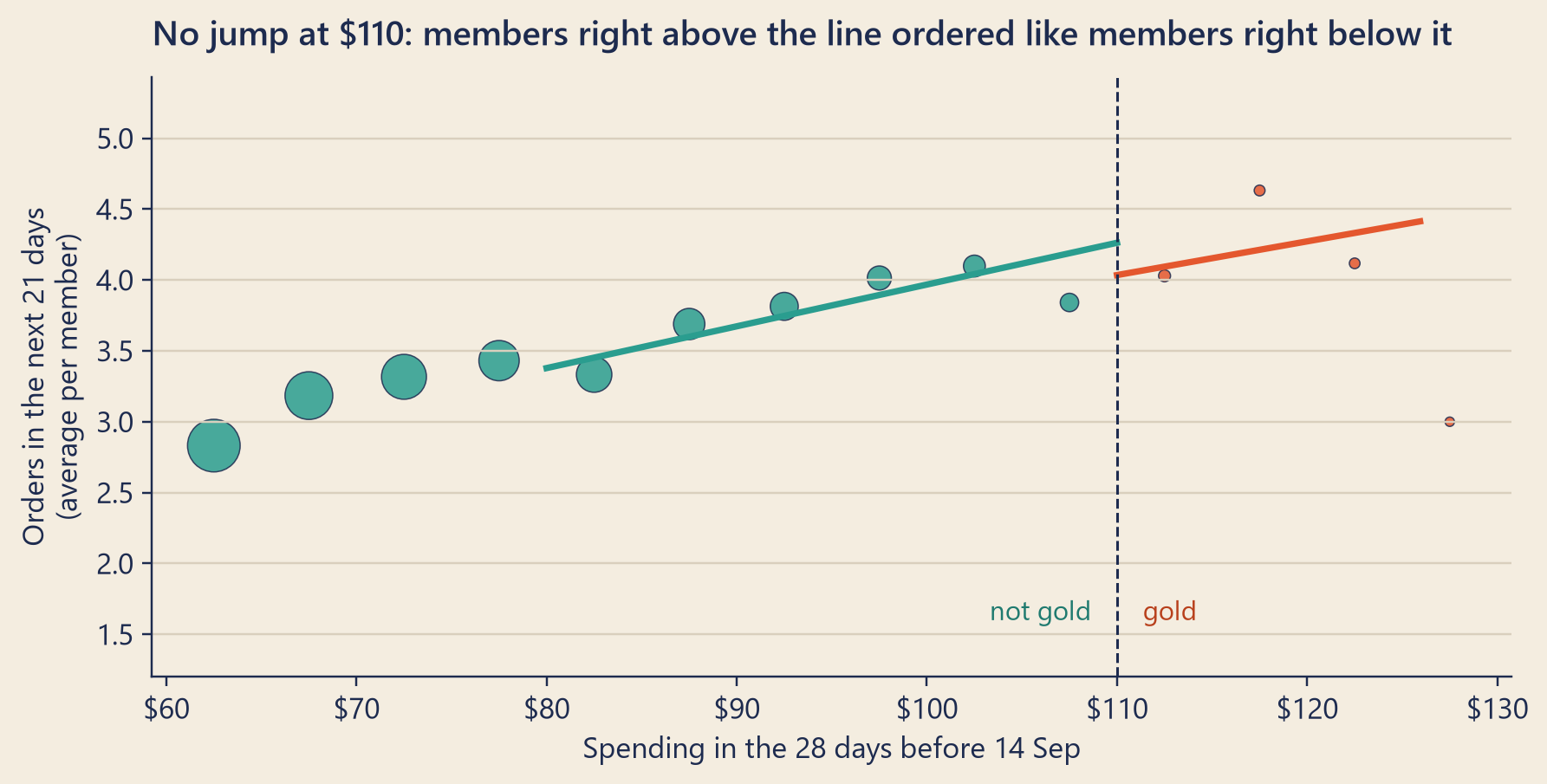
Figure 4: Members who were not gold on 13 September, by their spending from 17 August to 13 September, which the job used in the early hours of 14 September. Dots are averages per $5 band (bigger dots, more members). Lines are fitted within $30 on each side of the $110 line.

There is no jump. Right below the line, members ordered about 4.3 times in 21 days. The jump at $110 is −0.23 orders, with a 95% interval from −1.08 to +0.62 and p = 0.599.

The interval is wide: from about 25% fewer orders to 15% more, because only 72 members sit above the line. The job runs nightly. A member above $110 on an earlier night became gold then and is not in this group. Only members who crossed on the last day remain. So there is no sign that gold, by itself, changes how much people order, but too little data to rule out a modest effect. As Chapter 18 put it, “not guilty” is not “innocent”.

RD also needs the two sides of the line to be alike, apart from gold, and here they are not quite alike. Spending only rises on a day you order, so every member right above the line ordered on 13 September, the day they crossed. Only about a quarter of the members right below did. This RD is weaker evidence than it looks (Under the hood has the details).

For Priya, that means a lower bar for gold is not a proven way to get more orders. If she wants to know, she can test it, with a coin.

NoteUnder the hood

With \(x_i\) = spending minus $110 and \(G_i = 1\) when \(x_i \ge 0\), the local linear model, fitted only for members with \(|x_i| \le h\), is

\[\text{orders}_i = a + b\,x_i + \tau\,G_i + c\,x_i G_i + e_i.\]

The two sides get their own slopes, and \(\tau\) is the jump at the cutoff. Mia used \(h\) = $30 (2,302 members) and robust standard errors. A narrow window compares more similar people, but fewer of them. Bandwidths from $10 to $50 give jumps between −0.23 and +0.10 orders, all with intervals that include zero.

Checks. RD needs two things: people cannot place themselves exactly on one side of the line, and nothing else changes at it.

• Counts. Some members may buy one more drink to reach gold, which would pile them up above the line. Here the count falls instead, from 145 members at $105–110 to 34 at $110–115, by design (members already gold are left out), so a count cannot test for this.
• Traits gold cannot change. The share of iPhone users does not jump (p = 0.662). But “ordered on 13 September” does: 100% above the line against 26% within $30 below, a jump of 65 points in the model (p < 0.001).

Fuzzy over three weeks. On the morning of 14 September, the rule is sharp: every member at $110 or more became gold, and nobody below did. Over the 21 days of the outcome, it is not: 53% of members within $10 below the line became gold later. On average they spent 7.2 of the 21 days as gold, against 17.5 above the line. At the line, days as gold jump by 9.6 (standard error 0.8). When a cutoff changes only part of the treatment, the design is a fuzzy RD (Imbens and Lemieux, 2008), and its estimate divides the two jumps:

\[\hat\tau_{\text{fuzzy}} = \frac{\hat\tau_{\text{orders}}}{\hat\tau_{\text{gold days}} / 21}.\]

Fitted as a two-stage regression with robust errors, 21 full days of gold change orders by −12%, with a 95% interval from about −56% to +33%: this data cannot say much about gold. Either way, the answer is local: it describes members near $110.

Try it: move the window

viewof rdBand = Inputs.range([10, 50], {value: ch23.bandwidth, step: 5, label: "Window ($ each side)"})
viewof rdBin = Inputs.radio(new Map([["$2", 2], ["$5", 5], ["$10", 10]]), {value: 5, label: "Dot width"})

rdReadout = {
  const r = rdFit;
  const f = (x) => (x >= 0 ? "+" : "−") + Math.abs(x).toFixed(2);
  return html`<p>Members in the window: <strong>${r.n.toLocaleString("en-US")}</strong>
    (<strong>${r.nAbove}</strong> above the line). Right below the line: about
    <strong>${r.base.toFixed(1)}</strong> orders each in 21 days.</p>
    <p>Jump at $${ch23.gold}: <strong>${f(r.jump)}</strong> orders,
    95% interval ${f(r.lo)} to ${f(r.hi)}, p = ${r.p.toFixed(2)}.</p>`;
}

rdChart = {
  const C = {teal: "#2a9d8f", tomato: "#e4572e", ink: "#1d2b4f"};
  const g = ch23.gold, r = rdFit;
  const groups = d3.rollups(tierRows, (v) => ({n: v.length, y: d3.mean(v, (d) => d.y)}),
                            (d) => Math.floor(d.spend / rdBin) * rdBin + rdBin / 2);
  const dots = groups.map(([x, s]) => ({x, y: s.y, n: s.n, side: x >= g ? "gold" : "not gold"}));
  const xMaxAbove = d3.max(tierRows.filter((d) => d.spend >= g), (d) => d.spend) - g;
  const lines = [
    {side: "not gold", pts: [[-rdBand, r.a - r.b * rdBand], [0, r.a]]},
    {side: "gold", pts: [[0, r.a + r.jump], [Math.min(rdBand, xMaxAbove), r.a + r.jump + (r.b + r.c) * Math.min(rdBand, xMaxAbove)]]}
  ].flatMap((l) => l.pts.map(([x, y]) => ({side: l.side, x: g + x, y})));
  return Plot.plot({
    width: Math.max(300, Math.min(680, width)), height: 300, marginLeft: 46, marginBottom: 42,
    style: {background: "transparent", fontSize: "12px"},
    x: {label: "28-day spending ($)", labelAnchor: "center", labelOffset: 36, domain: [58, 130]},
    y: {label: "↑ Orders in next 21 days", domain: [0, 7], grid: true},
    r: {range: [1.5, 11]},
    color: {domain: ["not gold", "gold"], range: [C.teal, C.tomato], legend: true},
    marks: [
      Plot.rect([{x1: g - rdBand, x2: g + rdBand}], {x1: "x1", x2: "x2", fill: C.ink, fillOpacity: 0.05}),
      Plot.ruleX([g], {stroke: C.ink, strokeDasharray: "4,3"}),
      Plot.dot(dots, {x: "x", y: "y", r: "n", fill: "side", fillOpacity: 0.8, stroke: C.ink, strokeWidth: 0.5}),
      Plot.line(lines, {x: "x", y: "y", z: "side", stroke: "side", strokeWidth: 2.6})
    ]
  });
}

tierDb = DuckDBClient.of({tiers: FileAttachment("../data/out/web/tier_threshold.parquet")})
tierRows = {
  const rows = await tierDb.query(`select spend_28d::double as spend, orders_next_21d::double as y from tiers`);
  return rows.map((r) => ({spend: Number(r.spend), y: Number(r.y)}));
}
// Local linear RD: orders = a + b*x + jump*G + c*x*G within the window, robust (HC1) errors.
rdFit = {
  const near = tierRows.filter((d) => Math.abs(d.spend - ch23.gold) <= rdBand);
  const X = near.map((d) => { const x = d.spend - ch23.gold, G = x >= 0 ? 1 : 0; return [1, x, G, x * G]; });
  const y = near.map((d) => d.y);
  const n = near.length, k = 4;
  const xtx = [0, 1, 2, 3].map((i) => [0, 1, 2, 3].map((j) => X.reduce((s, row) => s + row[i] * row[j], 0)));
  const inv = invert(xtx);
  const xty = [0, 1, 2, 3].map((i) => X.reduce((s, row, t) => s + row[i] * y[t], 0));
  const beta = inv.map((row) => row.reduce((s, v, j) => s + v * xty[j], 0));
  const e2 = X.map((row, t) => (y[t] - row.reduce((s, v, j) => s + v * beta[j], 0)) ** 2);
  const meat = [0, 1, 2, 3].map((i) => [0, 1, 2, 3].map((j) => X.reduce((s, row, t) => s + row[i] * row[j] * e2[t], 0)));
  const mult = (A, B) => A.map((row) => B[0].map((_, j) => row.reduce((s, v, t) => s + v * B[t][j], 0)));
  const se = Math.sqrt(mult(mult(inv, meat), inv)[2][2] * n / (n - k)), z = 1.959964;
  return {n, nAbove: near.filter((d) => d.spend >= ch23.gold).length, a: beta[0], b: beta[1],
          jump: beta[2], c: beta[3], base: beta[0], lo: beta[2] - z * se, hi: beta[2] + z * se,
          p: twoSidedP(beta[2] / se)};
}

Matching and propensity scores

Why not compare gold members with other members directly? Mia did, on the same day. Over the next 21 days, gold members placed 5.4 orders each and everyone else 1.5. Nobody believes gold caused this: gold members are gold because they order a lot. When who gets the treatment depends on who they are, the groups differ before the treatment starts. This is called selection.

The standard repair is matching: compare each treated person with untreated people who look the same on the things you measured. Between $80 and $110 of 28-day spending, Steep has both kinds of member: 941 gold members who earned gold earlier and kept it, and 2,230 members who are not gold that day (most never reached $110; 830 had gold before and lost it). Mia put them into $5 bands of spending and compared gold with not gold inside each band.

Gold minus not gold, orders in the next 21 days	Gap	95% interval	Gold members compared
All members	+3.93	+3.82 to +4.05	2,683
Members with $80–$110 of spending	+1.07	+0.88 to +1.27	941
… matched on 28-day spending	+0.92	+0.72 to +1.13	941
… matched on 28-day spending and the 28 days before	−0.14	−0.40 to +0.15	831
A different group: members who crossed $110 that day (RD)	−0.23	−1.08 to +0.62	72

Matching on 28-day spending left a clear gap: about 0.92 more orders, with an interval above zero. It looks like proof that gold works. Then Mia added spending in the 28 days before that. The gold members had spent $95 on average in that earlier month, against $53 for the others. Matched on both months, the gap was gone. This is regression to the mean (Chapter 16): one month of spending is a noisy measure of usual spending. The gold member usually spends more and had a quiet month; the other usually spends less and had a busy one.

There is one more problem. Every one of these gold members was already gold during the month Mia matched on, half of them for 18 days or more. If gold made them order more, that extra spending is inside the number she matched on, and matching would hide it, on both matched lines. Match only on things measured before the treatment began.

That is the limit of every matching method: you can only match on what you measured, at the right time. In real problems, part of the difference is never recorded: a new job, a friend who loves tea.

With many traits, the cells of look-alike people soon run empty. A propensity score helps: each person’s chance of getting the treatment, predicted from all the measured traits (Rosenbaum and Rubin, 1983). You then match people with similar scores. It has the same limit. Matching makes groups alike in what you measured. A coin makes them alike in everything.

NoteUnder the hood

The matched gap averages the gap inside each cell \(s\), weighted by the gold members in it:

\[\hat\tau = \sum_s \frac{n_{1s}}{n_1}\left(\bar y_{1s} - \bar y_{0s}\right),\]

where \(n_{1s}\) is the number of gold members in cell \(s\), and \(\bar y_{1s}\), \(\bar y_{0s}\) are the average orders of gold and other members there. Cells without both kinds are dropped, so fewer gold members are compared on the last matched line. This is the effect on the treated. The intervals come from 1,000 bootstrap resamples of members.

The propensity score is \(e(x) = P(\text{treated} \mid X = x)\). Rosenbaum and Rubin showed this: if, among people with the same \(X\), who gets the treatment has nothing to do with how they would have done without it (no hidden confounders), the same is true among people with the same \(e(X)\). So matching on one number is enough. The “if” is the whole question: it cannot be tested from the data.

Two more needs. Overlap: every treated person needs untreated people with similar scores. At the sharp $110 line there is none: that night, nobody below the line became gold and everybody above did. That is why RD compares neighbours across the line instead. And the model that predicts the score can be wrong, so check that the traits are balanced after matching.

Common traps

• Choosing the comparison after seeing the answer. Try enough cities and windows, and one will say what you hoped. Fix them first; show the others as checks.
• Two changes on the same day. DiD gives the fee everything that hit Riverside alone from 5 October.
• A comparison group the change also touched. If Riverside shoppers had started ordering from Oldtown’s stores, Oldtown would be partly treated.
• Controlling for something the change itself moved. Do not put Riverside’s delivery fee or its checkout visits into the recipe. Control only for things the fee cannot change, such as rain.
• Reading “no jump” as “no effect”. Report the range, not only the point.

TipAudit Instinct · Peers and a second witness

Auditors rarely judge a branch’s numbers on their own. They compare it with similar branches in the same period: if every branch’s sales rose 2% and one branch’s fell 2%, that branch is where they look. That is difference-in-differences, done in the head.

They also want corroborating evidence: a second, independent source that tells the same story. Mia used a classic completeness test: check a numbered sequence for gaps. Steep’s order numbers come from one counter. Theo explained that the checkout takes the next number only at the payment screen, where Riverside shoppers saw the new fee; a customer who leaves there leaves a number unused. From 1 June to 4 October, there were no gaps. From 5 October to 25 October, 839 numbers were never used.

A missing number carries no city. But if each was a Riverside shopper who saw the fee and left, 839 of 21,466 would-be Riverside orders were lost (3.9%); the DiD said about 943. The gaps miss people the fee put off earlier and include people who came back later, so they could be bigger or smaller than the true loss. Still, two methods and two sources tell the same story: not proof, but a second witness.

NoteInterview Corner

1. What are the assumptions of difference-in-differences?

NoteA model answer

Parallel trends: without the treatment, both groups would have changed by the same amount on the scale you analyse (often logs, so the same percent). Also: no anticipation (nobody changed behaviour early because they knew the change was coming); no other change hitting only the treated group at the same time; no spillover to the comparison group. For the interval, allow for noise related from day to day, and beware of having few groups.

2. How do you check parallel trends?

NoteA model answer

Only before the change. Plot both groups over a long pre-period on the analysis scale and see whether they move together. Run placebo tests (fake start dates, or a fake treated group) and check that they find about zero. Then see whether the answer survives other reasonable windows and comparison groups.

3. When would you use regression discontinuity?

NoteA model answer

When a sharp rule on a measured score gives the treatment, such as a spending threshold. Compare units right above and below the cutoff, with a trend on each side. It needs units that cannot place themselves exactly on one side, and nothing else changing at the cutoff. Check that the number of units and unrelated traits do not jump there, and try several bandwidths. If the cutoff changes only part of the treatment, use a fuzzy RD. The answer is local to the cutoff.

4. What are the pitfalls of propensity score matching?

NoteA model answer

It balances only what you measured; hidden confounders remain, and you cannot test for them. It needs overlap: treated units with no comparable untreated units must be dropped, which changes who you describe. The score model can be wrong, so check balance after matching. Never match on things the treatment itself changed.

Reported change: −12.0% orders, the week of 7 September compared with the week before (CEO dashboard).

Explained so far: 12.0 of the 12 points, closed in Chapter 21: the tracking bug 7.0, the rainy week before 3.4, normal growth −0.3, and the price rise 1.9. Plus a new answer for the board, outside the twelve percent: the Riverside delivery fee cost about 4.5% of Riverside’s orders from 5 October (95% interval 2.6% to 6.4%), about 943 orders in three weeks.

Suspects: —

Ruled out: the matcha menu (Chapter 4); the data’s journey after the app (Chapters 8–14); Priya’s day-3 “win” (Chapter 21).

Open questions: how to tell the board of directors, on one page (Chapter 24).

New evidence: the comparison cities moved with Riverside all summer, fake start dates find nothing, and the order-number gaps point the same way. Separately, there is no sign that gold status alone changes how much members order, but that test is weak.

Recap

• Without a coin, look for a comparison group that went through the same weeks without the change, and compare changes, not levels. That is difference-in-differences.
• Check the comparison before the change (parallel trends) and on dates when nothing happened (placebo tests). Put measured confounders, like rain, into the recipe.
• A sharp rule can act almost like a local coin, if the two sides of the line are alike (regression discontinuity). Matching and propensity scores balance only what you measured before the treatment. Report ranges, including wide ones.

English	中文
causal inference	因果推断
observational data	观测数据
natural experiment	自然实验
counterfactual	反事实
causal diagram	因果图
confounding	混杂
difference-in-differences (DiD)	双重差分
comparison group	对照组 / 比较组
parallel trends	平行趋势
controlling for	控制（某变量）
placebo test	安慰剂检验
regression discontinuity (RD)	断点回归
running variable	驱动变量
cutoff	断点 / 阈值
selection	选择偏差
matching	匹配
propensity score	倾向得分
overlap	共同支撑 / 重叠
corroborating evidence	佐证

Further reading

• Card, D., & Krueger, A. B. (1994). Minimum Wages and Employment: A Case Study of the Fast-Food Industry in New Jersey and Pennsylvania. American Economic Review, 84(4), 772–793. RePEc
• Angrist, J. D., & Pischke, J.-S. (2009). Mostly Harmless Econometrics: An Empiricist’s Companion. Princeton University Press. DOI
• Imbens, G. W., & Lemieux, T. (2008). Regression Discontinuity Designs: A Guide to Practice. Journal of Econometrics, 142(2), 615–635. DOI
• Bertrand, M., Duflo, E., & Mullainathan, S. (2004). How Much Should We Trust Differences-in-Differences Estimates? The Quarterly Journal of Economics, 119(1), 249–275. DOI
• Conley, T. G., & Taber, C. R. (2011). Inference with “Difference in Differences” with a Small Number of Policy Changes. The Review of Economics and Statistics, 93(1), 113–125. DOI
• Rosenbaum, P. R., & Rubin, D. B. (1983). The Central Role of the Propensity Score in Observational Studies for Causal Effects. Biometrika, 70(1), 41–55. DOI
• Cunningham, S. (2021). Causal Inference: The Mixtape. Yale University Press. DOI. The author’s free online version is at mixtape.scunning.com, which now hosts the second edition, Causal Inference: The Remix, still in progress.