On the Monday of her third week, Mia found a message from Dana at the top of her inbox: For the board deck: September GMV so far. One number, please. By Wednesday.
GMV means gross merchandise value: the total value of the goods that customers bought. At Steep, the goods are cups of tea. It sounded like one simple sum.
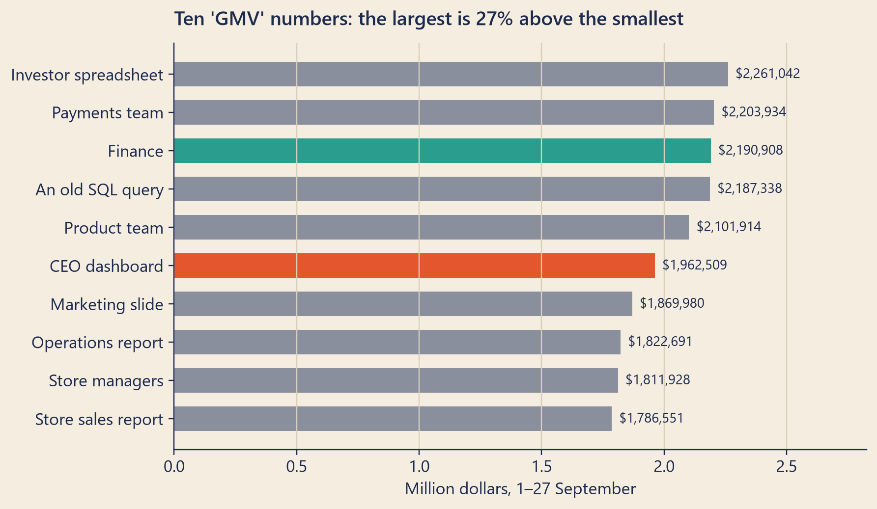
Mia searched Steep’s dashboards, reports and shared spreadsheets for “GMV” and “revenue” from 1 to 27 September. By lunch she had ten numbers. The smallest was $1,786,551. The largest was $2,261,042. Each number had an owner, and each owner was sure that their number was the right one.
She wrote all ten in her notebook, one per line. Next to each one she wrote the question from her first day: of what?
Theo stopped at her desk with a cup of coffee and read the list upside down.
“Ten,” he said. “Last year we had seven. We are growing.”
“Which one is right?”
“Each one answers its own question. That is the problem.” He took a napkin and drew four lines, one above the other. “Have you seen the back room of the big Harbor store?”
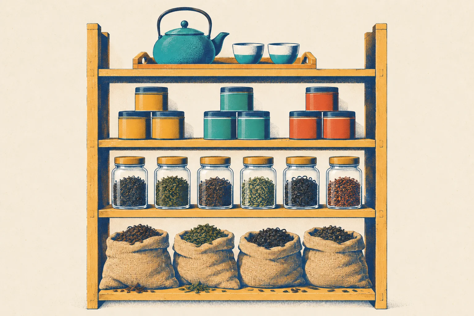
On the lowest line he drew sacks. On the next line, jars. Then small tins. On the top line, a tray with a teapot.
“Raw leaves arrive in sacks. Someone cleans and sorts them into jars. Someone else weighs portions into tins, one tin for each recipe. The tray goes to the customer. Each shelf takes only from the shelf below it. Nobody makes tea straight from a sack.”
“And my ten numbers?”
“Ten people took leaves from different shelves, weighed them on different scales, and gave the tea the same name.”
Mia wrote at the top of a new page: One name. One definition. One shelf.
ImportantThe big idea
Decide the grain of each table and the definition of each metric once, in one place. Then build everything else on top of them.
Look at the picture: the four shelves of a tea pantry. Sacks of raw leaves at the bottom. Jars of sorted leaves above them. Small tins in three colours above the jars. A serving tray at the top. A data warehouse is built the same way. By the end of this chapter, each shelf will have a name.
Ten numbers called GMV
Here is Mia’s list. Every number covers the same 27 days, 1 to 27 September, as Steep’s data stood at the end of Sunday, 27 September.
Table 1: Ten numbers called GMV or revenue, for 1–27 September. Days are Steep’s local days unless the row says otherwise.
Where Mia found it
What it adds up
1–27 Sep
CEO dashboard
Paid amount of orders with an order_completed event in the warehouse, refunds removed, by event day
$1,962,509
Marketing slide
Menu value of every order placed, cancelled ones too
$1,869,980
Operations report
Menu value of orders not cancelled
$1,822,691
Store managers
Menu value of completed orders, refunds removed
$1,811,928
Investor spreadsheet
Paid amount of every order placed
$2,261,042
Payments team
Paid amount of orders not cancelled (refunds not removed)
$2,203,934
Finance
Paid amount of completed orders, refunds removed
$2,190,908
Store sales report
Finance’s number without delivery fees
$1,786,551
Product team
Finance’s number without corporate bulk orders
$2,101,914
An old SQL query
Finance’s number, but with days counted in UTC
$2,187,338
Show the code
plot = variants.sort_values("amount")colors = [bk.TEAL if o =="Finance"else bk.TOMATO if o =="CEO dashboard"else bk.MUTED for o in plot.owner]fig, ax = bk.figure(8, 4.6)ax.barh(plot.owner, plot.amount /1e6, color=colors, height=0.65)for y, v inenumerate(plot.amount): ax.text(v /1e6+0.03, y, money(v), va="center", fontsize=9, color=bk.INK)ax.set_xlim(0, gmv_high /1e6*1.25)ax.set_xlabel("Million dollars, 1–27 September")ax.grid(axis="x", visible=True)ax.grid(axis="y", visible=False)ax.set_title(f"Ten 'GMV' numbers: the largest is {bk.fmt_pct(gmv_spread, 0)} above the smallest")plt.show()
Figure 1: The same ten numbers, sorted. Teal: finance’s number. Tomato: the CEO dashboard.
None of these numbers is a mistake. Each one is the right answer to a slightly different question. They differ in five choices, and you met most of them in Chapter 1.
Where it is counted. The CEO dashboard starts from app events. Everyone else starts from the orders database.
What counts. Are cancelled orders in? Are refunded orders in?
Which amount. The menu value (gross_amount) is the price of the drinks before any discount. The paid amount (net_amount) is what the customer paid: the menu value, minus discounts, plus the delivery fee. That is why a paid amount can be larger than a menu value.
Who. Corporate bulk orders (Chapter 2) are in or out.
When. Steep’s day starts at midnight in Steep’s cities. The old SQL query counts days in UTC, world standard time, which is 7 hours ahead. Its “1 September” starts at 17:00 on 31 August, Steep time.
And there is always an eleventh way. A finance team that subtracts each refund on the day the money goes back, not on the day of the order, gets $2,182,187.
The largest number is 27% above the smallest. If two reports to the board used two of these numbers, the board would see a gap that is not there.
There is no “true GMV” to find. The fix is to choose, to write the choice down, and to give each choice its own name. But first Mia needed the words that warehouse designers use.
Facts, dimensions and grain
Look at Mia’s receipt for A1024 again. It has numbers you can add up: one drink, a price, a total. And it has words that describe the order: which store, which day and time, which app, which way to pay. The two kinds of information have names.
A fact, or measure, is a number about a business event that you can add up or average: items, menu value, paid amount.
A dimension is the context of the event: who (the customer), where (the store, the city), when (the day, the hour), and how (the app, the payment method). You filter and group facts by dimensions: “paid amount by city”, “orders on iOS”.
A fact table holds one row for each business event, such as one order. Some fact tables hold one row per period instead, such as one day per city: a periodic snapshot fact table. A dimension table holds one row for each thing that gives context, such as one store or one customer.
The most important word in warehouse design is grain: what one row of a table stands for. You met it in Chapter 1 as “one row = one what?”. Ralph Kimball, who made this style of design popular, describes it as four steps, in this order:
Select the business process. (For Steep: customers placing orders.)
Declare the grain. (One row per order.)
Identify the dimensions. (Date, store, customer, app, payment method.)
Identify the facts. (Items, menu value, discount, delivery fee, paid amount.)
The order matters. If you choose columns before you declare the grain, you get a table where some rows are orders and some are order lines, and every sum becomes a trap: the fan-out of Chapter 3. Every table in Steep’s warehouse has a declared grain:
Table
One row is
dwd_order_detail
one fulfilled order (completed, or completed and later refunded)
dwd_event_detail
one app event
dws_city_platform_day
one day, in one city, on one platform
ads_ceo_dashboard_day
one day
Facts also differ in how they add up. Counts of events and sums of money are additive: you can add them across any dimension. Counts of different things, such as buyers, are not. A customer who buys on Monday and on Tuesday is one buyer, not two. Add up the buyers of every day, city and platform from 1 to 27 September, and you get 162,360. The real number of different buyers is 59,746.
Ratios, such as an average order value, are non-additive too. In September, dws_city_platform_day has 324 rows, one per day, city and platform. Take each row’s average order value and average them, and you get $13.98. Divide the total paid amount by the total number of orders, and you get $12.61. The first method gives a quiet day of Riverside web orders the same weight as a busy day of Harbor iOS orders. So store the parts, the sums and the counts, and divide at the end.
A third kind, semi-additive, adds up across some dimensions but not across time. Steep’s loyalty program, which you will meet below, puts its members in tiers, and gold is the top one. You can add Harbor’s gold members to Riverside’s. You cannot add Monday’s gold members to Tuesday’s: most are the same people.
Stars and wide tables
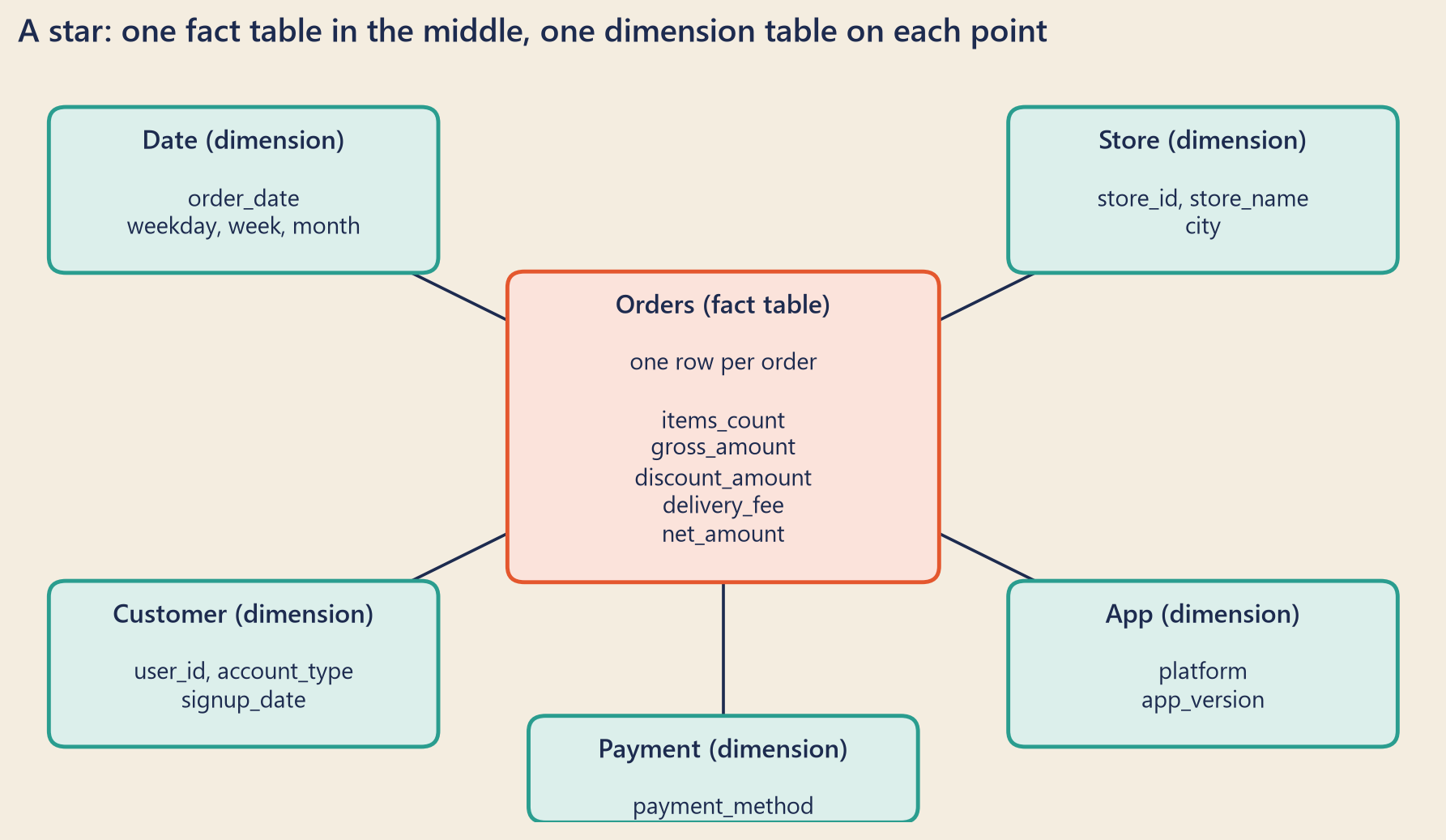
Put the order fact table in the middle and its dimension tables around it, and the drawing looks like a star. This layout is called a star schema.
Show the code
bk.setup()fig, ax = plt.subplots(figsize=(8, 4.6), layout="constrained")ax.set_xlim(0, 100)ax.set_ylim(0, 57)ax.axis("off")ax.set_title("A star: one fact table in the middle, one dimension table on each point")def star_box(cx, cy, w, h, title, body, edge, face): ax.add_patch(FancyBboxPatch((cx - w /2, cy - h /2), w, h, boxstyle="round,pad=0.3,rounding_size=1.2", linewidth=1.6, edgecolor=edge, facecolor=face, zorder=2)) ax.text(cx, cy + h /2-1.4, title, ha="center", va="top", fontsize=10.5, fontweight="semibold", color=bk.INK, zorder=3) ax.text(cx, cy + h /2-5.6, body, ha="center", va="top", fontsize=9.5, color=bk.INK, linespacing=1.3, zorder=3)fact_xy = (50, 30)dims = [((16, 48), "Date", "order_date\nweekday, week, month"), ((84, 48), "Store", "store_id, store_name\ncity"), ((16, 12), "Customer", "user_id, account_type\nsignup_date"), ((84, 12), "App", "platform\napp_version"), ((50, 4), "Payment", "payment_method")]for (x, y), _, _ in dims: ax.plot([fact_xy[0], x], [fact_xy[1], y], color=bk.INK, linewidth=1.2, zorder=1)star_box(*fact_xy, 30, 23, "Orders (fact table)","one row per order\n\nitems_count\ngross_amount\ndiscount_amount\ndelivery_fee\nnet_amount", bk.TOMATO, "#fbe3db")for (x, y), title, body in dims: h =7.5if title =="Payment"else12 star_box(x, y, 27, h, f"{title} (dimension)", body, bk.TEAL, "#dcefeb")plt.show()
Figure 2: Steep’s orders as a star schema. The fact table holds the numbers; each dimension table describes one side of the order.
To ask for “paid amount by city on iOS last week”, a query joins the fact table to the store and date dimensions, filters, and groups. It needs one join per dimension. The queries are short and fast, and a beginner can read them.
Big-data warehouses often go one step further. They copy the most useful dimension columns into the fact table itself, so that most questions need no join at all. A table like that is a wide table. Steep’s dwd_order_detail is one: next to each order it keeps the store’s name and the customer’s account type and signup date. The cost: a bigger table, and copied names that can get old. Steep’s real nightly pipeline rewrites only yesterday’s partition (Chapter 13), so an old order keeps the store name it had on the night it was written. build_layers.sql, the script that builds this book’s copy of the warehouse, rebuilds every table in one go, because the dataset is small; there, every row gets today’s name. Know which kind you have.
Notice one column that is not in the wide table: the customer’s loyalty tier. Tiers change every night. You will see below how a warehouse keeps them.
NoteUnder the hood
Snowflakes. Suppose the store dimension does not hold the city’s name. It holds a city number, and a separate city table holds the names. The dimension has been split into smaller tables, like the branches of a snowflake. This layout is a snowflake schema. It stores each city name only once, but every question about cities needs one more join. Kimball advises against it: a flat dimension holds the same information, and it is easier to read and usually faster.
A grain test. A table’s grain is a promise: one row per key. Test it with count(*) = count(DISTINCT (order_date, city, platform)). Chapter 13 shows a day when that promise broke.
Four shelves: ODS, DWD, DWS, ADS
Steep’s warehouse is built in four layers, like the pantry. It follows a naming style that is common in Chinese data teams and was made popular by Alibaba: every table name starts with its layer.
Table 2: The four shelves of Steep’s warehouse, from the bottom up. Row counts are real, up to 27 September.
build_layers.sql has one rule: each layer reads only from layers below it, never from one above. ADS may read DWS or DWD; nothing above DWD reads raw ODS. There is one exception, in the playground. Here is a short tour, with real excerpts.
ODS keeps the raw data. For orders, it does not even copy the files. It points at the folders that the lake already holds (Chapter 9):
DWD cleans. It keeps only orders that were fulfilled, and it removes the copies of events that Kafka delivered twice (Chapter 8). QUALIFY keeps one row per event_id: the one with the lowest offset, its position number in Kafka.
CREATEORREPLACETABLE dwd_event_detail ASWITH deduplicated AS (SELECT*FROM ods_events QUALIFY row_number() OVER (PARTITIONBY event_id ORDERBY"offset") =1)
DWS summarises. Its orders are completed orders that were not refunded:
CREATEORREPLACETABLE dws_city_platform_day ASSELECT order_date, city, platform,count(*) FILTER (WHERENOT is_refunded) AS orders,-- ...FROM dwd_order_detailGROUPBY order_date, city, platform
ADS serves. Each ADS table is made for one report or one team. You will read the dashboard’s SQL in a moment.
Why go to all this trouble?
Clean once, use many times. Kafka’s copies are removed in one place, not in every report.
A change in a source touches one shelf. If the app renames an event, only one DWD job changes.
Summaries are cheap.dws_city_platform_day answers daily questions with 1,428 rows instead of 751,272.
You can follow any number down to its raw rows. The map of which table is built from which is called lineage.
The price is more tables, more jobs to run, and data that arrives a little later.
Two notes on names. Many teams add a fifth layer, DIM, for shared dimension tables such as users and stores. Alibaba Cloud’s DataWorks lists ODS, DIM, DWD, DWS and ADS as its built-in layers. A dimension that every fact table shares, with the same keys and the same meaning, is a conformed dimension: one store table, one definition of a city. It is half of the cure for ten GMVs: every report groups by the same stores. And teams that use the medallion architecture speak of bronze (raw data), silver (cleaned data) and gold (data shaped for reports), with no link to the loyalty tiers below. Roughly, bronze is ODS, silver is DWD, and gold is DWS and ADS. The mapping is approximate, because every team draws the lines in a slightly different place.
Following the dashboard down the shelves
Before she chose any GMV, Mia wanted to understand the number that started the whole case: the “orders” on Dana’s wall. She followed it down, shelf by shelf. Here is the top of ads_ceo_dashboard_day, exactly as it is in build_layers.sql:
CREATEORREPLACETABLE ads_ceo_dashboard_day ASWITH completed_events AS (SELECT event_date, order_idFROM dwd_event_detailWHERE event_name ='order_completed'),-- ... e.event_date,count(*) AS orders,-- ...FROM completed_events AS e
There it was, in plain SQL. The dashboard’s “orders” is a count of order_completedevents. It is not a count of rows in the orders database. One shelf down, the events come from dwd_event_detail. One more shelf down, from ods_events. Below that, from Kafka, and from the app on each customer’s phone. This is the root of the confusion: the most important number in the company was defined, years ago, on the top shelf, from the wrong sack.
Did the shelves lose anything on the way up? In the two weeks of the case, ODS holds 88,213 different order_completed events. DWD holds the same number, and so does the dashboard. The shelves lost nothing. The recipe on the top shelf used the wrong ingredient.
Mia wrote her proposal on one page:
Orders are counted from the orders database: completed orders that were not refunded, from dwd_order_detail through dws_city_platform_day. App events are still counted, under their own name: “order_completed events”.
For the case, the two definitions tell two stories. These are the numbers as Mia saw them on Monday (the case board uses final statuses, see Chapter 1):
Week
Dashboard today (events)
Mia’s proposal (orders database)
The week before, 31 Aug–6 Sep
46,924
45,548
The week of the drop, 7–13 Sep
41,289
43,326
Change
−12.0%
−4.9%
In the week before the drop, the dashboard is higher than the database. It counts every order that sent the event, including orders that were later cancelled or refunded (Chapter 1). From 7 September it is lower, because some orders sent no event at all. Over 1–27 September, the dashboard counts 159,968 orders and the database 173,739.
Dana read the page twice. “So the database line goes to the board.”
“Yes. The database is the book of record: it is where the money is. The event line measures the app’s tracking. That is useful too, but it is a different thing.”
“Change it,” said Dana. “But keep both lines on my wall, with honest names, until we know why they differ.”
A table that remembers
Priya had one more request for Mia’s list: “orders from gold members”, for her product report.
Steep Rewards started on 1 June. Every member starts at bronze. Each night at 02:15, a job looks at the member’s completed spending over the last 28 days and sets the tier for the new day: bronze, silver or gold.
The users table keeps only today’s tier. When a member moves from gold to silver, the word “gold” is overwritten and gone. That is fine for “which tier is this member today?” It is wrong for “how many of last week’s orders came from gold members?”, because some members were gold last week and are silver today, and others the other way round.
A dimension whose values change from time to time is a slowly changing dimension, or SCD. Kimball numbers the ways to handle one. These four are the common ones:
Type 0: keep the original. The value never changes, like a signup date.
Type 1: overwrite. Keep only today’s value. History is lost.
Type 2: add a row. Each change adds a new row, a new version, with the dates when it was true. History is kept.
Type 3: add a column. Keep today’s value and the one before it, side by side. One step of history.
The choice between type 1 and type 2 changes real answers. Last week, 21 to 27 September, members who were gold on the day they ordered placed 4,671 orders. Ask the type 1 question, “orders from members who are gold today”, and the answer is 5,694: 22% more. The difference is in who moved. 1,182 of those orders came from members who were not yet gold when they ordered and were gold by Sunday; only 159 went the other way. Tiers rise with spending, so the members who ordered a lot last week are the ones who moved up, and type 1 counts their earlier orders as gold.
The zipper table
Steep keeps tier history as type 2, in dwd_user_zipper. Chinese data teams call this design a zipper table (拉链表). Each version of a member’s tier is one row, with a start_date, the first day it was true, and an end_date, the last day it was true. The version that is still true gets the end date 9999-12-31, a date far in the future that means “until further notice”, and is_current is true. Each version ends exactly one day before the next one starts, so the rows close up like the teeth of a zipper: no gaps and no overlaps.
Here is one member, u100676, as the warehouse saw them on Monday morning. Every night, Steep also saves a full copy of the users table, in ods_users_snapshot. First, the member in those nightly copies, 21 to 27 September:
Table 3: One member in seven nightly copies of the users table (ods_users_snapshot).
Night (dt)
loyalty_tier
2026-09-21
gold
2026-09-22
gold
2026-09-23
silver
2026-09-24
silver
2026-09-25
silver
2026-09-26
silver
2026-09-27
silver
Seven rows that mostly repeat each other. Now the same member in the zipper table, for the whole summer:
Table 4: The same member in the zipper table (dwd_user_zipper), as known on 27 September.
loyalty_tier
start_date
end_date
is_current
bronze
2026-06-01
2026-06-12
false
silver
2026-06-13
2026-06-22
false
gold
2026-06-23
2026-09-22
false
silver
2026-09-23
9999-12-31
true
Four rows tell the whole story. The member was gold from 23 June and became silver on 23 September. The nightly copies show only the end of it: gold on the first nights of the week, silver after that.
To ask “which tier on 15 August?”, pick the row whose dates contain that day:
SELECT loyalty_tierFROM dwd_user_zipperWHERE user_id ='u100676'ANDDATE'2026-08-15'BETWEEN start_date AND end_date;
To get every member’s tier today, ask for the rows with end_date = DATE '9999-12-31'.
Size explains why teams like zipper tables. A full copy every night from 1 June to 27 September would hold 9,169,494 rows. The zipper table holds the same history in 197,425 rows, about 46 times fewer.
Steep builds the zipper from ods_user_tier_changes, a table of every tier change and its date. By 27 September it held 86,298 enrolments and 111,127 tier changes. The zipper can also be built from the nightly copies. Mia built it both ways: over 21 to 27 September, both give the same 92,918 rows, with 0 differences. A check of the whole zipper (no gaps, no overlaps, one current row per member, and agreement with every nightly copy) found 0 problems. After that, a job runs every night: it closes the open row of each member whose tier changed, and opens a new one. The box below shows both ways to build a zipper and the nightly job, as SQL that is tested each time this book is built.
NoteUnder the hood
Building it from the change table. Each change starts a version, and a version ends the day before the next one starts. This is the real SQL from build_layers.sql:
CREATEORREPLACETABLE dwd_user_zipper ASWITH versions AS (SELECT user_id, new_tier AS loyalty_tier, effective_date AS start_dateFROM ods_user_tier_changes)SELECT user_id, loyalty_tier, start_date,coalesce(lead(start_date) OVER by_user -1, DATE'9999-12-31') AS end_date,lead(start_date) OVER by_user ISNULLAS is_currentFROM versionsWINDOW by_user AS (PARTITIONBY user_id ORDERBY start_date)ORDERBY user_id, start_date;
lead() is a window function (Chapter 3). It looks at the next row of the same member.
Building it from nightly copies. For one member, let \(x_t\) be the tier on night \(t\). Mark each night whose tier differs from the night before, and number the versions with a running total:
where \(\mathbf{1}[\cdot]\) is 1 when the condition is true and 0 otherwise (the first night always counts as a change). Nights with the same \(v_t\) form one version; collapse each version into one row. This is dwd_user_zipper_from_snapshots. A member who goes gold, then silver, then gold again gets three versions, not two. That is why you cannot group by tier alone.
The nightly job. It reads last night’s zipper and tonight’s copy of the users table. It closes the open row of every member whose tier changed, and of every member who left, and it opens a new row for each changed or new member. Keep each night’s zipper as its own partition. Tonight’s job reads last night’s partition and overwrites tonight’s, so a rerun gives the same answer. (Chapter 13 calls this idempotent.) With only one copy, a second run starts from the first run’s result, and changes the rows again. Classic Hive tables cannot change one row in place anyway (Chapter 11), so the job writes a whole new partition. In the SQL, UNION ALL stacks the rows of two queries, and INSERT OVERWRITE replaces a whole partition (Chapter 13 explains it):
-- Tonight's job for 2026-09-27. Each night's zipper is its own partition (dt).WITH yesterday AS ( -- last night's zipperSELECT user_id, loyalty_tier, start_date, end_dateFROM dwd_user_zipperWHERE dt =DATE'2026-09-27'-1),today AS ( -- every member's tier tonightSELECT user_id, loyalty_tierFROM ods_users_snapshotWHERE dt =DATE'2026-09-27'AND loyalty_tier ISNOTNULL),closing AS ( -- open rows whose member changed tier, or leftSELECT y.user_idFROM yesterday AS yLEFTJOIN today AS t USING (user_id)WHERE y.end_date =DATE'9999-12-31'AND (t.user_id ISNULLOR t.loyalty_tier <> y.loyalty_tier)),opening AS ( -- new members, and members whose tier changedSELECT t.user_id, t.loyalty_tierFROM today AS tLEFTJOIN yesterday AS yON y.user_id = t.user_id AND y.end_date =DATE'9999-12-31'WHERE y.user_id ISNULLOR y.loyalty_tier <> t.loyalty_tier)INSERT OVERWRITE TABLE dwd_user_zipper PARTITION (dt ='2026-09-27')-- 1. Every row from last night; the open rows in "closing" end yesterday.SELECT y.user_id, y.loyalty_tier, y.start_date,CASEWHEN c.user_id ISNOTNULLTHENDATE'2026-09-27'-1ELSE y.end_date ENDAS end_date, y.end_date =DATE'9999-12-31'AND c.user_id ISNULLAS is_currentFROM yesterday AS yLEFTJOIN closing AS cON c.user_id = y.user_id AND y.end_date =DATE'9999-12-31'UNIONALL-- 2. One new open row for each member in "opening".SELECT user_id, loyalty_tier, DATE'2026-09-27', DATE'9999-12-31', trueFROM opening;
Mia ran it for the night of 27 September, on the zipper as it stood the night before. It found 1,404 members to update: 1,260 tier changes and 144 new members. Its result matched dwd_user_zipper row for row, and a second run gave the same rows again. She also tried it on a tiny made-up night, with one member who left, one who moved up and one who joined. All three came out right.
The nightly job cannot fix a change dated before a member’s current row starts. You rebuild that member’s history from the change table. That is one more reason to keep it.
Why 9999-12-31, and not an empty end date? With a real date in every row, one test, d BETWEEN start_date AND end_date, finds the version true on day \(d\), including the current one. With an empty (NULL) end date, every query needs coalesce(end_date, ...) first. Some teams store half-open intervals instead: the end date is the first day the version is no longer true, and the test becomes start_date <= d AND d < end_date. Both work. Pick one, write it down, and test it, because mixing them creates one-day gaps or overlaps.
Joining facts to a type 2 dimension. This chapter joins orders to tiers by date: o.order_date BETWEEN z.start_date AND z.end_date. Kimball’s classic design gives each version its own surrogate key, a new ID made by the warehouse, and stores in each fact row the key of the version that was true when the order happened. Then the join is a plain =.
The other types. Kimball’s list goes on to type 7. Type 4 moves attributes that change often into a small separate dimension, and types 5 to 7 mix the others.
One name, one definition: the metric layer
Back to Dana’s question. Mia’s real fix was not a table. It was a list.
A metric dictionary gives each metric one name, one written definition, one owner, and one place where it is computed. When a dashboard needs “net revenue”, it does not write its own SUM. It asks for the metric by name, and adds its own filters, such as a city or a week. The part of a data platform that holds these definitions and computes them is the metric layer, also called the semantic layer. Some teams buy a tool for it. Mia started with a shared page and one SQL view per metric. Here are the first three entries in her dictionary:
Name
Definition
Day
Computed from
1–27 Sep, on Monday
orders
Completed orders, refunded ones removed
local order day
dws_city_platform_day
173,739
net_revenue
Paid amount (after discounts, with delivery fee) of completed orders, refunded ones removed
local order day
dws_city_platform_day
$2,190,908
gmv
Menu value (before discounts, without delivery fee) of orders not cancelled; refunds not removed
local order day
dwd_order_detail
$1,822,691
That afternoon, Mia sent Dana a draft slide with two numbers, GMV and net revenue. Under each one, in small print, was its definition. Dana replied with one line: “First time a footnote made me believe a number. Keep doing that.”
NoteUnder the hood
The parts of a metric. Alibaba Cloud’s DataWorks breaks a metric into parts. The parts help even without the tool.
An atomic metric says what to measure and how: “paid amount of completed orders”.
A time period says when: “the last 7 days”.
A modifier narrows the scope: “on iOS”, “in Harbor”.
A derived metric is an atomic metric plus a time period plus modifiers: “paid amount of completed orders, last 7 days, on iOS”.
Ten dashboards can ask for ten derived metrics and still share one atomic definition.
Try it
The first playground is the zipper table of real Steep members, as the warehouse knew them on the night of 27 September. Change a tier, and watch rows close and open.
The zipper-table builder. Pick a member. The strip shows them in seven nightly copies of the users table; the table and the timeline show their zipper rows. Then give them a new tier from some day, and press “Apply the change”. Rows that were closed turn mustard; new rows turn teal.
zipperBuilder = {const C = {teal:"#2a9d8f",tealText:"#1f7a6f",tomatoText:"#b8401c",mustard:"#f2b134",ink:"#1d2b4f",paper:"#f4ede0",deep:"#ebe2d0",muted:"#8a8f9e",white:"#fffdf8"};const TIER = {bronze: {fill:"#d9a77a",letter:"B"},silver: {fill:"#cfd2db",letter:"S"},gold: {fill: C.mustard,letter:"G"}};const OPEN ="9999-12-31", DAY =86400000, f = ch12;const toMs = s =>Date.UTC(+s.slice(0,4),+s.slice(5,7) -1,+s.slice(8,10));const iso = ms =>newDate(ms).toISOString().slice(0,10);const addDays = (s, n) =>iso(toMs(s) + n * DAY);const plain = rows =>Array.from(rows, r => (typeof r.toJSON==="function"? r.toJSON() : r));const memberIn = Inputs.select(newMap(f.presets.map(p => [`${p.user}: ${p.why}`, p.user])), {label:"Member"});const tierIn = Inputs.radio(["bronze","silver","gold"], {label:"New tier",value:"gold"});const dateBox = htl.html`<input type="date" class="zb-date" min=${f.start} max=${f.dataEnd} value=${f.today}>`;const askBox = htl.html`<input type="date" class="zb-date" min=${f.start} max=${f.dataEnd} value="2026-08-15">`;let user =null, rows = [], start = [], snaps = [], marks =newMap(), note ="", sql ="";asyncfunctionload(id) { user = id;const z =plain(await zipDb.query(` SELECT loyalty_tier AS tier, CAST(start_date AS VARCHAR) AS s, CASE WHEN end_date >= DATE '${f.knownUntil}' THEN '${OPEN}' ELSE CAST(end_date AS VARCHAR) END AS e FROM zipper WHERE user_id = '${id}' AND start_date <= DATE '${f.knownUntil}' ORDER BY start_date`)); snaps =plain(await zipDb.query(` SELECT CAST(dt AS VARCHAR) AS dt, loyalty_tier AS tier FROM snaps WHERE user_id = '${id}' ORDER BY dt`)); rows = z.map(r => ({tier: r.tier,start: r.s,end: r.e})); start = rows.map(r => ({...r})); marks =newMap(); sql =""; note =`${rows.length} zipper row${rows.length===1?"":"s"} for ${id}, `+`as the warehouse knew them on ${f.knownUntil}.`; }functionrebuild(versions) {const merged = [];for (const v of versions) {if (!merged.length|| merged[merged.length-1].tier!== v.tier) merged.push(v); }return merged.map((v, i) => ({tier: v.tier,start: v.start,end: i +1< merged.length?addDays(merged[i +1].start,-1) : OPEN})); }functionapply() {const day = dateBox.value, tier = tierIn.value;if (!rows.length) { note ="This member has no rows to change.";return; }if (!day || day <= rows[0].start) { note =`Pick a day after ${rows[0].start}, the day this member joined.`;return; }const open = rows[rows.length-1];const forward = day > open.start;if (forward && tier === open.tier) { note =`${user} is already ${tier}. The nightly merge finds no difference, so it writes nothing.`; marks =newMap(); sql ="";return; }const before = rows;const versions = before.filter(r => r.start!== day).map(r => ({start: r.start,tier: r.tier})); versions.push({start: day, tier}); versions.sort((a, b) => (a.start< b.start?-1:1)); rows =rebuild(versions);if (JSON.stringify(rows) ===JSON.stringify(before)) { note =`Nothing changed: on ${day}, ${user} was already ${tier}, so the rows stay as they were.`; marks =newMap(); sql ="";return; }const same = r => before.some(b => b.start=== r.start&& b.tier=== r.tier&& b.end=== r.end);const closed = r => before.some(b => b.start=== r.start&& b.tier=== r.tier&& b.end!== r.end); marks =newMap(rows.map((r, i) => [i,same(r) ?"":closed(r) ?"closed":"new"]));if (forward) { note =`The open row ended on ${addDays(day,-1)}, and a new open row starts on ${day}. `+"Nothing else moved. This is what the nightly merge does for one member."; sql =`-- The night of ${day}, for one member: close the open row, then open a new one.UPDATE dwd_user_zipperSET end_date = DATE '${addDays(day,-1)}', is_current = falseWHERE user_id = '${user}' AND end_date = DATE '${OPEN}';INSERT INTO dwd_user_zipper (user_id, loyalty_tier, start_date, end_date, is_current)VALUES ('${user}', '${tier}', DATE '${day}', DATE '${OPEN}', true);`; } else { note =`This change is dated before the open row began (${open.start}). The rows around `+`${day} were rebuilt from the change log. The nightly merge cannot do this.`; sql =`-- A backdated change: add it to the change log, then rebuild this member from the log.DELETE FROM dwd_user_zipper WHERE user_id = '${user}';INSERT INTO dwd_user_zipperSELECT user_id, new_tier, effective_date, coalesce(lead(effective_date) OVER w - 1, DATE '${OPEN}'), lead(effective_date) OVER w IS NULLFROM ods_user_tier_changesWHERE user_id = '${user}'WINDOW w AS (PARTITION BY user_id ORDER BY effective_date);`; } }functionchecks() {const chain = rows.every((r, i) => i ===0|| r.start===addDays(rows[i -1].end,1));const current = rows.filter(r => r.end=== OPEN).length;const ok = chain && current ===1;return`${ok ?"✓":"✗"} No gaps and no overlaps: ${chain ?"yes":"no"}. `+`Current rows: ${current} (should be 1).`; }// --- drawing ------------------------------------------------------------------------------const strip = htl.html`<div class="zb-strip"></div>`;const tableBox = htl.html`<div class="zb-table"></div>`;const timeBox = htl.html`<div class="zb-time"></div>`;const noteBox = htl.html`<div class="zb-note" aria-live="polite"></div>`;const checkBox = htl.html`<div class="zb-check"></div>`;const askOut = htl.html`<div class="zb-ask" aria-live="polite"></div>`;const sqlBox = htl.html`<pre class="zb-sql"></pre>`;functiondrawStrip() { strip.replaceChildren(...snaps.map(s => htl.html`<div class="zb-night" style="background:${TIER[s.tier] ? TIER[s.tier].fill: C.deep}"> <span class="zb-day">${+s.dt.slice(8,10)} Sep</span> <strong>${TIER[s.tier] ? TIER[s.tier].letter:"–"}</strong></div>`));if (!snaps.length) strip.textContent="This member is not in the nightly copies of 21-27 September."; }functiondrawTable() { // built with DOM calls: a bare <tr> in a template can be droppedconst table =document.createElement("table");const row = (cells, tag, cls) => {const tr =document.createElement("tr");if (cls) tr.className= cls;for (const c of cells) {const td =document.createElement(tag); td.textContent= c; tr.appendChild(td); }return tr; };const head =document.createElement("thead"); head.appendChild(row(["loyalty_tier","start_date","end_date","is_current",""],"th"));const body =document.createElement("tbody"); rows.forEach((r, i) => {const mark = marks.get(i) ||""; body.appendChild(row([r.tier, r.start, r.end, r.end=== OPEN ?"true":"false", mark],"td", mark ?"zb-"+ mark :"")); }); table.append(head, body); tableBox.replaceChildren(table); }functiondrawTimeline() {const W =Math.max(300,Math.min(720, timeBox.clientWidth||640));const L =8, R =8, H =74, y =22, h =26;const t0 =toMs(f.start), t1 =toMs(f.dataEnd) + DAY;const x = s => L + (W - L - R) * (Math.min(toMs(s), t1) - t0) / (t1 - t0);const shapes = []; rows.forEach((r, i) => {const x1 =x(r.start), x2 = r.end=== OPEN ? W - R :x(addDays(r.end,1));const mark = marks.get(i); shapes.push(htl.svg`<rect x=${x1} y=${y} width=${Math.max(1, x2 - x1)} height=${h} fill=${TIER[r.tier].fill} stroke=${mark ==="new"? C.teal: mark ==="closed"? C.mustard: C.ink} stroke-width=${mark ?3:0.8} />`);if (x2 - x1 >14) { shapes.push(htl.svg`<text x=${(x1 + x2) /2} y=${y +17} text-anchor="middle" font-size="12" font-weight="600" fill=${C.ink}>${TIER[r.tier].letter}</text>`); } });for (const m of ["06","07","08","09","10"]) {const xm =x(`2026-${m}-01`); shapes.push(htl.svg`<line x1=${xm} x2=${xm} y1=${y + h} y2=${y + h +5} stroke=${C.ink} />`); shapes.push(htl.svg`<text x=${xm +2} y=${y + h +17} font-size="11" fill=${C.ink}>${ ["Jun","Jul","Aug","Sep","Oct"][+m -6]}</text>`); }const xt =x(f.today); shapes.push(htl.svg`<line x1=${xt} x2=${xt} y1=${y -8} y2=${y + h +2} stroke=${C.ink} stroke-dasharray="3 3"/>`); shapes.push(htl.svg`<text x=${xt} y=${y -10} text-anchor="middle" font-size="11" fill=${C.ink}>${+f.today.slice(8,10)} Sep</text>`);const xa =x(askBox.value|| f.start); shapes.push(htl.svg`<path d="M ${xa -5}${y -9} L ${xa +5}${y -9} L ${xa}${y -2} Z" fill=${C.tomatoText} />`); timeBox.replaceChildren(htl.svg`<svg viewBox="0 0 ${W}${H}" width=${W} height=${H} role="img" aria-label=${`Timeline of ${user}'s tier versions from June to October`} style="max-width:100%;font-family:Inter,system-ui,sans-serif">${shapes}</svg>`); }functionask() {const d = askBox.value;const hit = rows.findIndex(r => r.start<= d && d <= r.end); askOut.textContent=!d ?"": hit <0?`On ${d}, ${user} was not a member yet: no row contains that day.`:`On ${d}, ${user} was ${rows[hit].tier}: row ${hit +1}, because `+`${rows[hit].start} ≤ ${d} ≤ ${rows[hit].end}.`; }functionrender() {drawStrip();drawTable();drawTimeline();ask(); noteBox.textContent= note; checkBox.textContent=checks(); sqlBox.textContent= sql ||"-- Apply a change to see the SQL that would make it."; }const button = (label, action) => {const b = htl.html`<button type="button" class="zb-btn">${label}</button>`; b.addEventListener("click",async () => { awaitaction();render(); });return b; }; memberIn.addEventListener("input",async () => { awaitload(memberIn.value);render(); }); askBox.addEventListener("input", () => { drawTimeline();ask(); });const resizer =newResizeObserver(() =>drawTimeline()); resizer.observe(timeBox); invalidation.then(() => resizer.disconnect());awaitload(memberIn.value);render();const style =document.createElement("style"); style.textContent=` .zb-wrap { font-family: Inter, system-ui, sans-serif; color: ${C.ink}; } .zb-row { display: flex; flex-wrap: wrap; gap: 0.4rem 1rem; align-items: center; margin: 0.4rem 0; } .zb-date { font: 0.9rem Inter, system-ui, sans-serif; padding: 0.2rem 0.3rem; border: 1px solid ${C.muted}; border-radius: 4px; background: ${C.white}; color: ${C.ink}; } .zb-btn { font: 600 0.85rem Inter, system-ui, sans-serif; color: ${C.paper}; background: ${C.ink}; border: 0; border-radius: 5px; padding: 0.45rem 0.8rem; cursor: pointer; } .zb-btn:hover { background: ${C.teal}; } .zb-btn:focus-visible { outline: 3px solid ${C.mustard}; outline-offset: 2px; } .zb-label { font-size: 0.82rem; font-weight: 600; } .zb-strip { display: flex; flex-wrap: wrap; gap: 0.3rem; margin: 0.3rem 0 0.6rem; } .zb-night { width: 3.3rem; border: 1px solid ${C.ink}; border-radius: 4px; text-align: center; font-size: 0.75rem; padding: 0.15rem 0; } .zb-night strong { display: block; font-size: 1rem; } .zb-table { overflow-x: auto; max-width: 100%; } .zb-table table { border-collapse: collapse; font-size: 0.8rem; margin: 0.3rem 0; } .zb-table th, .zb-table td { border-bottom: 1px solid rgba(29, 43, 79, 0.15); padding: 0.2rem 0.5rem; text-align: left; white-space: nowrap; } .zb-table tr.zb-new td { background: rgba(42, 157, 143, 0.22); } .zb-table tr.zb-closed td { background: rgba(242, 177, 52, 0.35); } .zb-time { width: 100%; margin: 0.2rem 0; } .zb-note, .zb-check, .zb-ask { font-size: 0.85rem; margin: 0.3rem 0; } .zb-note { min-height: 2.6em; } .zb-sql { font: 0.74rem/1.4 "JetBrains Mono", Consolas, monospace; background: ${C.deep}; color: ${C.ink}; padding: 0.6rem; border-radius: 5px; overflow-x: auto; max-width: 100%; white-space: pre; margin-top: 0.4rem; }`;return htl.html`<div class="zb-wrap">${style}${memberIn} <div class="zb-label">Seven nightly copies of the users table (B = bronze, S = silver, G = gold)</div>${strip} <div class="zb-label">The zipper rows</div>${tableBox}${timeBox}${checkBox} <div class="zb-row">${tierIn}</div> <div class="zb-row"><span class="zb-label">From the day</span> ${dateBox}${button("Apply the change", apply)}${button("Start again",async () => { awaitload(user); })}</div>${noteBox}${sqlBox} <div class="zb-row"><span class="zb-label">Which tier on</span> ${askBox}</div>${askOut} </div>`;}
Things to try:
With the first member, give them gold from 1 October. One row closes, one opens.
Now give them bronze from 1 August. The change is dated in the past, so several rows change. This is why a zipper is rebuilt from the change log when history is corrected.
Ask for a day before the member joined. No row contains it.
Pick the member who changed most often, and count the nightly copies against the zipper rows.
The second playground is a map of Steep’s real tables. Pick any table to see what it is built from and what is built from it.
The lineage explorer. Shelves run from the serving tray at the top to the sources at the bottom, as in the picture. Pick a table: the tables it reads from turn tomato, the tables that read from it turn teal. Then switch the definition of the dashboard’s orders.
Start at ads_ceo_dashboard_day. Its orders climb down through dwd_event_detail and ods_events to the app. Now switch to Mia’s proposal: the path runs through dws_city_platform_day and dwd_order_detail to the main database, and the change in the case weeks moves with it.
Pick ods_events and see how much depends on one raw table.
Pick ads_experiment_user. It reads the raw ods_users table directly, which the rule forbids. Real warehouses have exceptions like this one. A good team writes them down.
Common traps
One name, many definitions. “GMV”, “revenue” and even “orders” mean nothing until the definition is written next to them.
A table with two grains. Orders and order lines in one table make every sum a trap. Declare the grain, then test it: one row per key.
Averaging averages. Store sums and counts. Divide at the end.
Type 1 history. Joining old orders to today’s tier rewrites the past. Last week’s gold orders went from 4,671 to 5,694.
A broken zipper. Gaps, overlaps, two current rows, or a backdated change merged as if it were new. Run the same checks every night that Mia ran once.
Reading the raw shelf from the top. An ADS table that reads raw ODS data skips the cleaning in DWD. If you must do it, write down why.
TipAudit Instinct · The chart of accounts, and the vendor master file
Your books are layered too. Source documents become journal entries. Journals post to the general ledger. The ledger is summed into a trial balance, and the trial balance becomes the financial statements. Each layer is built only from the one below, and an auditor can trace any line in the statements down to its documents. That is ODS, DWD, DWS and ADS, long before computers. A group of companies adds one more step, consolidation: each company’s accounts are mapped to one group chart of accounts before anything is added up.
The chart of accounts is a metric dictionary. “Revenue” in the statements has one account code, one owner and one written rule for what goes in. Nobody in finance invents their own revenue for a slide. A metric dictionary brings the same habit to dashboards.
A zipper table is a master-data change log. Auditors review changes to the vendor master file, above all changes to bank accounts, a classic route for fraud. The test question is: “Which bank account did this vendor have on the day we paid?” A system that overwrites the account (type 1) cannot answer. A history table with valid-from and valid-to dates (type 2) can.
NoteInterview Corner
Q1. Why do we build a warehouse in layers, such as ODS, DWD, DWS and ADS? (为什么要分层?)
NoteA short answer
Each layer has one job. ODS keeps a raw copy, so you can always rebuild. DWD cleans and standardises at the finest grain. DWS builds shared summaries at common grains. Each ADS table is made for one report or one team. The benefits: clean once and reuse many times; a change in a source touches one layer; any number can be traced down (lineage); summaries make common questions cheap; and each layer has a clear owner. Without layers, every report reads raw data on its own, a style Chinese teams call “chimney” development (烟囱式开发). The costs are more tables, more jobs and more delay. Each layer reads only from layers below it, and exceptions are written down.
Q2. Write SQL to build a zipper table, and to update it every night. (拉链表怎么实现?)
NoteA short answer
Build: from a table of every change and its date, keep one change per member per day (two changes on the same day would give a row whose end_date is before its start_date), give each change a row and end it the day before the member’s next change: coalesce(lead(start_date) OVER (PARTITION BY user_id ORDER BY start_date) - 1, DATE '9999-12-31'). From daily full copies of the table, mark the nights where the value changed, number the versions with a running sum, and group each version into one row. Update: keep one partition per night. Read last night’s partition and compare tonight’s copy with its open rows (end_date = '9999-12-31'). Close the open row of each member who changed or left; open a new row for each member who changed or joined; stack the two parts with UNION ALL and INSERT OVERWRITE tonight’s partition. A rerun reads the same inputs and writes the same partition. The full query is in the Under the hood box of “A table that remembers”. Use:WHERE d BETWEEN start_date AND end_date for “as of day d”. Test: no gaps, no overlaps, never two open rows for one member, and an open row for every member in tonight’s copy (a member who left has none). A backdated change needs a rebuild from the change table.
Q3. Star schema or snowflake schema? (星型模型和雪花模型的区别?)
NoteA short answer
A star joins the fact table directly to flat dimension tables: one join per dimension, simple queries, fast. A snowflake splits dimensions into smaller tables (store, then city, then region): less repetition and one place to change an attribute, but more joins and harder queries. Kimball recommends stars. Column stores compress repeated values well, so a snowflake saves little space. Many big-data teams go further than a star and copy dimension columns into wide tables in DWD and DWS.
Reported change: −12.0% orders, the week of 7 September compared with the week before (CEO dashboard).
Explained so far: 0 of the 12 points. About 7 of them sit between the orders database and the dashboard (Clue 1).
Suspects: the app, and the service that writes to Kafka (Chapter 8). The iOS app, version 3.2.0, is the main suspect (Chapter 6). Not proved.
Ruled out: the matcha menu (Chapter 4), Kafka (Chapter 8), storage (Chapter 9), computing (Chapter 10), refunds and restatements (Chapter 11), and now the warehouse layers. They pass every event up faithfully: all 88,213 order_completed events of the two case weeks reached the dashboard.
Open questions: which orders have no order_completed event, and why? Did iOS 3.2.1, released on 24 September, fix it? How many of the 12 points does it explain? (Chapter 15.)
New evidence: the dashboard’s “orders” is defined on the top shelf, in ads_ceo_dashboard_day, as a count of order_completed app events. Counted from the orders database, the same weeks show −5.0% (final statuses, see Chapter 1). From now on, Mia’s metric dictionary defines orders from the database, and Dana’s wall will show both lines, with honest names.
Recap
A metric is a definition. Write it down once, give it a name, and compute it in one place: the metric layer. Ten reports gave ten “GMV” numbers because nobody had.
Declare each table’s grain first. Facts are numbers about events; dimensions describe the events. A star schema keeps questions short.
Layers (ODS → DWD → DWS → ADS) clean data once and make every number traceable. Following Dana’s orders down the shelves showed that they were defined from app events. A zipper table (SCD type 2) keeps history as versions with a start date and an end date.
English
中文
gross merchandise value (GMV)
商品交易总额 / 成交总额
fact table
事实表
dimension table
维度表
measure
度量
grain
粒度
additive / semi-additive / non-additive fact
可加 / 半可加 / 不可加度量
conformed dimension
一致性维度
star schema
星型模型
snowflake schema
雪花模型
wide table
宽表
ODS (operational data store)
贴源层 / 操作数据层
DWD (data warehouse detail)
明细层
DWS (data warehouse summary)
汇总层
ADS (application data service)
应用层
DIM (dimension layer)
维度层
medallion architecture (bronze / silver / gold)
奖章架构(铜 / 银 / 金)
lineage
血缘
slowly changing dimension (SCD)
缓慢变化维
periodic snapshot fact table
周期快照事实表
daily full copy of a table
每日全量快照
zipper table
拉链表
change table / change log
变更表 / 变更日志
surrogate key
代理键
metric layer / semantic layer
指标层 / 语义层
metric dictionary
指标字典
atomic metric / derived metric
原子指标 / 派生指标
modifier / time period
修饰词 / 时间周期
Further reading
Ralph Kimball and Margy Ross, The Data Warehouse Toolkit: The Definitive Guide to Dimensional Modeling, 3rd edition, Wiley, 2013. The standard book on facts, dimensions, grain and slowly changing dimensions.
Kimball Group, “Dimensional Modeling Techniques”. Short official pages on the four-step process, grain, star schemas, snowflaking and each SCD type.
Alibaba Cloud DataWorks documentation: “Data warehouse layering” (ODS, DIM, DWD, DWS and ADS) and “Data metric” (atomic metrics, modifiers, time periods and derived metrics).