On Friday afternoon, Dana came to Mia’s desk with two cups of tea. That morning, Mia had rebuilt Dana’s chart for the board: two lines, the dashboard and the orders database, which part on 7 September (Chapter 5).
“The chart is good,” said Dana. “But I know my board. Before they look at any chart, one of them will ask me a question.” She put one cup down. “Are we losing customers?”
Mia thought about it. “Losing them where?”
“What do you mean, where?”
“There are two ways to lose a customer,” said Mia. “You can lose them at the door: they open the app, look around, and leave without buying. Or you can lose them over time: they buy once and never come back. Those are different problems. They need different pictures.”
She drew two shapes in her notebook. The first was a cone, wide at the top and narrow at the bottom. The second was a grid, with rows of different lengths.
Theo looked over from the next desk. “A funnel and a cohort table,” he said. “Two of the most useful charts in product analytics. Use the events_daily table for the funnel. For the cohorts, use the orders database, not the events.” He paused. “You know why.”
Mia did. Since Monday, the app’s events had been her main suspect. She wrote at the top of a new page: Are we losing customers? At the door: funnel. Over time: cohorts.
ImportantThe big idea
A funnel shows where people stop. A cohort shows whether they come back. Look at both before you say “we are losing customers”.
Look at the picture above. On the left, tea leaves pour into a glass funnel. Each of its four sections is narrower than the one before, so fewer leaves get through each one, and only a thin stream reaches the cup. On the right, four tea plants stand in a row, each planted at a different time. The funnel is this chapter’s first picture: where people stop. The plants are its second: groups that started at different times, and how they grow.
A funnel: where people stop
Steep’s app sends an event at five moments in a visit. The Prologue called them taps. Here are their names:
app_open: the customer opens the app.
view_menu: they open a store’s menu.
add_to_cart: they put a drink in the cart.
checkout_start: they go to the payment screen.
order_completed: they pay, and the order is placed.
Between the five events there are four steps. They are the four sections of the funnel in the picture, and the cup at the bottom is order_completed.
A funnel counts how many people reach each step of a process, in order. To build one, you must first decide what one “person” is. Mia used sessions. A session is one visit to the app, from opening it to leaving it. One customer can have many sessions in a week. For each step, she counted the sessions that reached it. Here is the week before the drop, 31 August to 6 September, on all platforms together:
Step
Sessions
Of the step before
Of all sessions
app_open
132,843
100.0%
view_menu
107,089
80.6%
80.6%
add_to_cart
77,023
71.9%
58.0%
checkout_start
59,775
77.6%
45.0%
order_completed
46,924
78.5%
35.3%
Two kinds of conversion
The table has two columns of rates, and they answer two questions.
The step conversion rate is the share of sessions at one step that also reached the next. Of the sessions that opened the payment screen, 78.5% ended in an order. (To be exact, the rate divides two counts: sessions with an order by sessions at the payment screen. It works as a share because almost every session with an order, 99.7%, also opened the payment screen.) This number tells you how well one step works.
The overall conversion rate is the share of all sessions that got this far. Of all the sessions that opened the app, 35.3% ended in an order. This number tells you how well the whole journey works.
The two are linked. To get the overall rate, you multiply the step rates together: 80.6% × 71.9% × 77.6% × 78.5% = 35.3%. Sessions that stop between two steps are the drop-off of that step.
When the overall rate falls, the step rates tell you where. That is the whole reason to build a funnel.
Split the funnel
A funnel for all of Steep is a mix of three apps: iOS, Android and the web. On Thursday, Priya’s matcha chart had reminded Mia how a total can hide its parts (Chapter 4). So she built one funnel per platform, for each week, and compared the week before with last week:
Step
iOS
Android
Web
to view_menu
81.2% → 81.2%
80.0% → 79.7%
79.7% → 79.3%
to add_to_cart
73.2% → 72.8%
70.4% → 69.9%
70.5% → 70.9%
to checkout_start
78.9% → 78.3%
76.1% → 75.3%
75.7% → 75.4%
to order_completed
80.0% → 69.0%
76.4% → 75.8%
76.7% → 76.1%
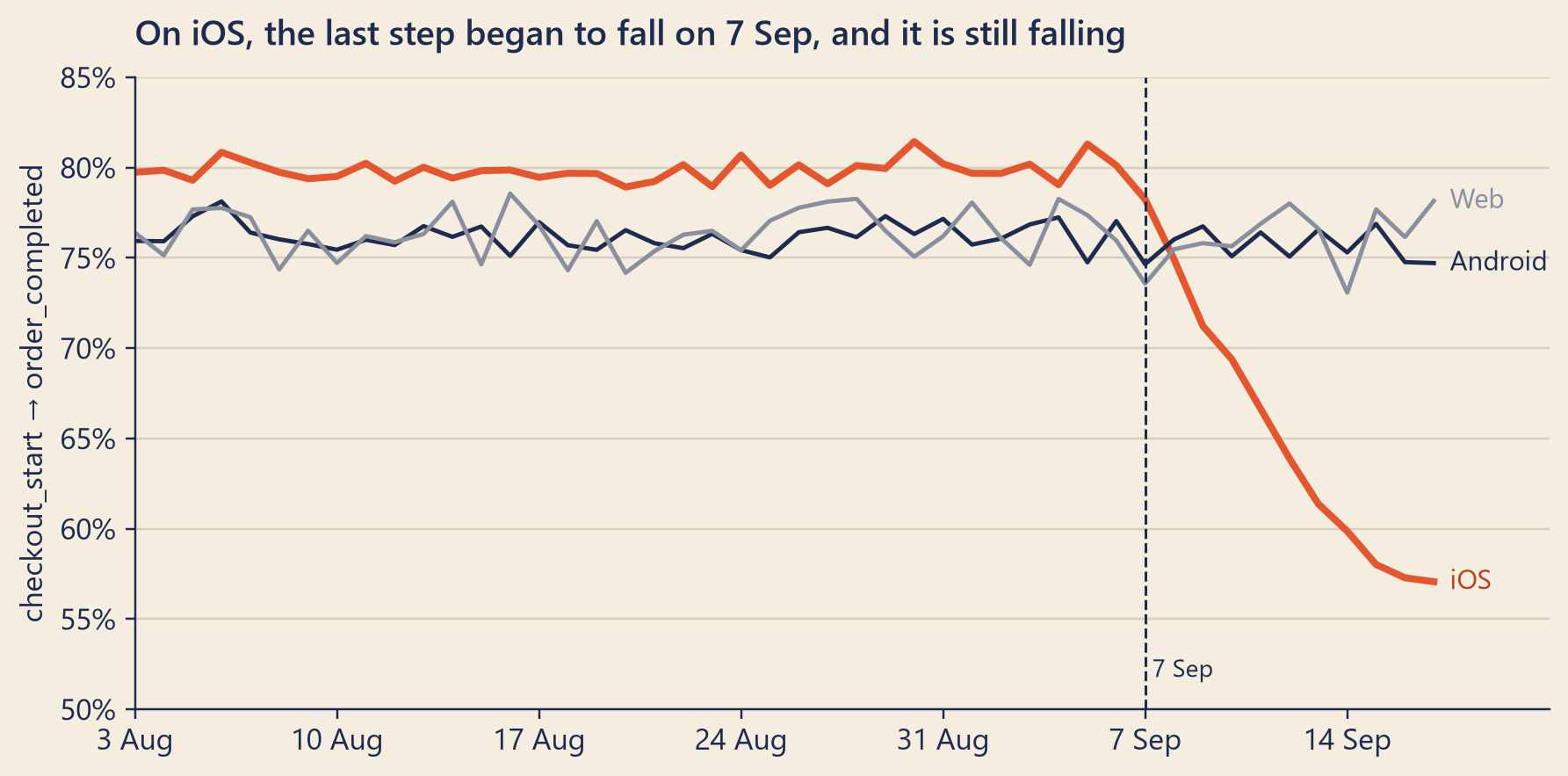
Twelve step rates. Eleven of them moved by less than one point. One of them collapsed: on iOS, the step from checkout_start to order_completed fell from 80.0% to 69.0%.
Customers on iPhones opened the app, looked at menus, filled their carts and reached the payment screen as often as before. Then, at the last moment, far fewer of them seemed to pay. On Android and the web, the last step barely moved.
Mia drew the last step day by day:
Show the code
fig, ax = bk.figure(8, 3.9)styles = {"ios": (bk.TOMATO, 2.6), "android": (bk.INK, 1.6), "web": (bk.MUTED, 1.6)}for p in PLATFORMS: d = daily[daily.platform == p] color, lw = styles[p] ax.plot(d.day, d.last_step, color=color, lw=lw) ax.annotate(PLATFORM[p], (d.day.iloc[-1], d.last_step.iloc[-1]), xytext=(6, 0), textcoords="offset points", va="center", fontsize=10, color=TOMATO_TEXT if p =="ios"else color)ax.axvline(W2_START, color=bk.INK, ls="--", lw=1)ax.text(W2_START, 0.515, f" {short(W2_START)}", fontsize=9, va="bottom")ax.set_ylim(0.5, 0.85)ax.yaxis.set_major_formatter(lambda v, _: f"{v:.0%}")ax.set_xlim(daily.day.min(), daily.day.max() + pd.Timedelta(days=4))mondays = pd.date_range(daily.day.min(), THROUGH, freq="W-MON")ax.set_xticks(mondays, [short(d) for d in mondays])ax.set_ylabel("checkout_start → order_completed")ax.set_title(f"On iOS, the last step began to fall on {short(W2_START)}, and it is still falling")plt.show()
Figure 1: The last step of the funnel, day by day: each day, the number of sessions with an order_completed event, divided by the number with a checkout_start event. The dashed line marks 7 September.
Until 6 September, the iOS line stayed between 78.9% and 81.4%. On 7 September it began to slide, a little more each day. On Thursday 17 September, it was 57.1%. For this week so far, Monday to Thursday, the step stood at 58.0%. Whatever happened was getting worse, not better.
The orders were there
Customers do not suddenly refuse to pay on one kind of phone, from one particular day, at one step only. Mia had seen patterns like this in her audit years. When one control fails on one system from one date, the first suspect is the system, not the people.
There was a simple way to check. The funnel’s last step counts order_completedevents: the app’s message that an order was paid. But every paid order also lands in the orders database. Mia replaced the bottom of the funnel with the database. For iOS, she divided the orders placed in the database by the sessions that reached the payment screen:
iOS, week
Sessions at checkout
order_completed events per checkout
Orders in the database per checkout
31 Aug – 6 Sep
34,184
80.0%
80.2%
7 Sep – 13 Sep
32,725
69.0%
79.5%
14 Sep – 17 Sep
17,855
58.0%
79.8%
Counted from the database, the last step did not move: it stayed between 79.5% and 80.2%. (This is a rough check. It divides orders by sessions, two different units, but one paid session makes one order, so the two should agree. Before the drop, they did.)
So iPhone customers kept paying. The orders were there. What was missing was their order_completed event in the warehouse. A funnel built from events can only see what the events see. Here it was looking at the same gap as the dashboard.
Mia asked Theo whether anything had changed on iOS on 7 September. He opened the release calendar. Two new versions had come out early that morning, and both changed the checkout: the iPhone app 3.2.0 and the website web-3.2. On the web, the last step barely moved: 76.7% the week before, 76.1% last week. So a new checkout does not, on its own, make the last step fall. Mia wrote in her notebook: Suspect: iOS app 3.2.0. Not proved. A date that fits is not yet a cause.
Cohorts: do they come back?
The funnel answered half of Dana’s question. Customers were not leaving at the door: they came in, filled their carts and paid. But were they coming back?
A cohort is a group of customers who started at the same time. Mia used the week of each customer’s first completed order. Everyone whose first order fell in the week of 13 July is one cohort. Everyone whose first order fell in the next week is the next cohort.
For each cohort, she asked: what share of these customers placed an order again, one week later? Two weeks later? Ten? This share is called retention. Each customer’s weeks are counted from their own first order. Week 0 is the first seven days, week 1 the next seven, and so on. A customer counts as retained in a week if they were an active customer that week: they placed at least one completed order, counted in the orders database.
Mia took the orders from the database, not from the app’s events, as Theo had said. The reason is in her notebook. From the week before to last week, active iPhone customers fell by 2.0%. Counted from order_completed events instead of the database, the same number fell by 13.0%. A cohort table built on the events would have shown customers leaving who had not left.
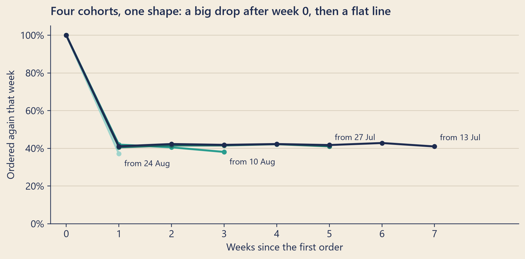
Here are four cohorts, two weeks apart. Like the four plants in the picture, each one is older than the next, so each one has more weeks behind it:
Show the code
fig, ax = bk.figure(8, 3.9)shades = ["#9fd4cc", bk.TEAL, "#1f6f66", bk.INK] # light to dark: youngest to oldestfor cohort, color inzip(sorted(FOUR, reverse=True), shades): d = first[first.cohort_week == cohort] ax.plot(d.weeks_since, d.retention, color=color, lw=2.2, marker="o", ms=4.5) below = cohort >= youngest - pd.Timedelta(weeks=2) # the two youngest: label under the line ax.annotate(f"from {short(cohort)}", (d.weeks_since.iloc[-1], d.retention.iloc[-1]), xytext=(6, -14if below else7), textcoords="offset points", fontsize=9, color=bk.INK)ax.set_ylim(0, 1.05)ax.yaxis.set_major_formatter(lambda v, _: f"{v:.0%}")ax.set_xticks(range(0, int(four.weeks_since.max()) +1))ax.set_xlim(-0.3, four.weeks_since.max() +1.6)ax.set_xlabel("Weeks since the first order")ax.set_ylabel("Ordered again that week")ax.set_title("Four cohorts, one shape: a big drop after week 0, then a flat line")plt.show()
Figure 2: Retention of four cohorts (by week of first order), as known on Friday 18 September. Only weeks that are fully over are shown.
Week 0 is always 100%. That is not a result; it is the definition. Everybody in a cohort ordered in their first week, or they would not be in it. The real story starts in week 1. There, the four cohorts drop to about 40%. After that, the lines run flat. Every week from week 1 on, in all four cohorts, sits between 37.2% and 42.8%, with an average of 41%.
A line like this is a retention curve. Many apps show the same shape: a big drop early on, then a line that falls more slowly and flattens. In the first-order view, the drop after week 0 is mostly built in: everyone in a cohort ordered in week 0. After that, Steep’s curve is flat. Each cohort orders at about the same rate, week after week. In many real apps, the curve keeps falling for several weeks, or months, before it flattens, because customers drift away a few at a time. Steep’s flat curve is good news, and it is also worth watching. (What a flat curve does and does not tell you is in the box “Under the hood” below.)
Mia tried a second start date: the week each customer signed up, whether they had ordered yet or not. In that view there is no early drop at all. About 33% of a cohort orders in week 0, and about 37% in every later week. That confirms it: the big drop in the first view comes from how the cohort is defined. The shape of a retention curve depends on how you define the start. Always say which one you used.
Reading a cohort table
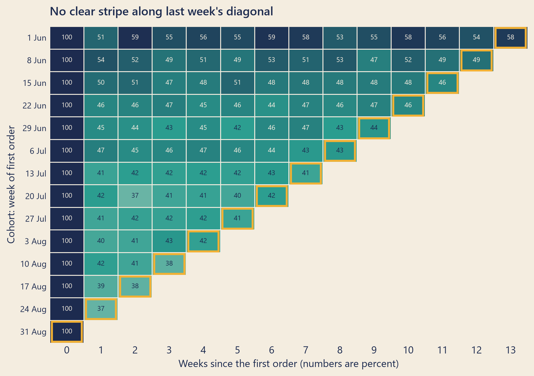
A retention curve shows a few cohorts. A cohort table shows all of them at once: one row per cohort, one column per week since the start. Each cell holds the retention of that cohort in that week. Colour the cells by their value, and you have a heatmap.
Show the code
cmap = LinearSegmentedColormap.from_list("steep", ["#efe6d4", bk.TEAL, bk.INK])norm = Normalize(0.25, 0.60, clip=True)cohorts =sorted(first.cohort_week.unique())max_k =int(first.weeks_since.max())fig, ax = bk.figure(8, 5.6)for row, cohort inenumerate(cohorts):for cell in first[first.cohort_week == cohort].itertuples(): color = cmap(norm(cell.retention)) ax.add_patch(Rectangle((cell.weeks_since, row), 1, 1, facecolor=color, edgecolor=bk.PAPER, lw=1)) ax.text(cell.weeks_since +0.5, row +0.5, f"{100* cell.retention:.0f}", ha="center", va="center", fontsize=7.5, color=bk.PAPER if norm(cell.retention) >0.55else bk.INK)if cell.last_week: ax.add_patch(Rectangle((cell.weeks_since +0.06, row +0.06), 0.88, 0.88, fill=False, edgecolor=bk.MUSTARD, lw=2.2))ax.set_xlim(0, max_k +1)ax.set_ylim(len(cohorts), 0)ax.set_xticks([k +0.5for k inrange(max_k +1)], range(max_k +1))ax.set_yticks([r +0.5for r inrange(len(cohorts))], [short(c) for c in cohorts], fontsize=9)ax.tick_params(length=0)ax.grid(False)for side in ("left", "bottom"): ax.spines[side].set_visible(False)ax.set_xlabel("Weeks since the first order (numbers are percent)")ax.set_ylabel("Cohort: week of first order")ax.set_title("No clear stripe along last week's diagonal")plt.show()
Figure 3: Mia’s cohort table on Friday 18 September: the share of each cohort (by week of first order) with a completed order in each later week. Outlined cells include days from last week, 7 to 13 September.
The table is a staircase. The oldest cohort has the longest row, because it has lived the longest; the newest has a single cell. It is the row of plants in the picture, turned on its side. Only finished weeks are shown. On Friday, the newest cohort’s second week was not over yet, so it has no cell.
You can read a cohort table in three directions:
Along a row, you follow one cohort as it gets older. This is its retention curve.
Down a column, you compare cohorts at the same age. Are newer customers better or worse than older ones?
Along a diagonal, from bottom left to top right, you see one stretch of calendar time, as every cohort lived through it. A problem that hits everybody at once, such as an outage, a strong competitor or a wave of customers leaving, shows up as a stripe along a diagonal.
That last direction is the one for Dana’s question. The outlined cells include days from last week, 7 September to 13 September. If many customers had left, the outlined cells would form a pale stripe. There is no clear stripe. But each cell mixes days from different calendar weeks, because every customer’s weeks start on their own first-order day. So Mia also measured last week directly, in calendar weeks.
She took the customers in the table whose first order was before 17 August. (She left out later ones. A customer’s first week counts automatically, so she made sure that no one’s first week, or the week right after it, fell in the two weeks she compared.) In the week before, 44.25% of them placed a completed order. Last week, 42.04% did: 2.2 points lower, or 5.0% fewer customers. A fall of about two points is too faint to see in the colours of the table. That is why there is no clear stripe.
The table holds only customers who signed up on or after 1 June. So Mia did the same for every customer who had ordered between 1 June and 16 August: 40.53% ordered in the week before and 38.87% last week. That is 1.7 points lower, or 4.1% fewer customers.
That is about the size of the real drop in orders, 5% (Chapter 1), which is still part of the case; Parts III and IV take it up. So: no sign yet that customers left. Fewer of them ordered last week, by about as much as the real drop. With data up to Thursday, a customer who left last week looks just like one who skipped a week. Whether they come back, the next weeks will show.
(The cohort files use final statuses; see Chapter 1. With the statuses Mia saw on Thursday, no cell moves by more than 0.5 of a point.)
Why not just count active customers?
Counting active customers, as defined above, is a fine first look. But a total like this can hide a lot. It mixes old customers with new ones, and new ones can cover up old ones who leave. Churn is the loss of customers who stop buying, and a total can hide churn for a long time.
Here is a made-up shop (not Steep). It wins 100 new customers every week, but it keeps few of them: 40% order again in their second week, 25% in their third, 15% in their fourth, 10% in their fifth, and 8% in their sixth.
Week
New customers
Active customers
Week 1
100
100
Week 2
100
140
Week 3
100
165
Week 4
100
180
Week 5
100
190
Active customers grow every week: from 100 to 190. The chart on the wall would look great. Yet each cohort loses most of its customers within two weeks. If new customers stopped coming in week 6, only the old cohorts would be left: 40 + 25 + 15 + 10 + 8 = 98 active customers, at once. A cohort table shows the leak as soon as the first cohorts are a few weeks old. A total shows it only when the new customers stop.
NoteUnder the hood
Step rates multiply. Write \(N_0, N_1, \dots, N_4\) for the sessions that reach each step. The step rate is \(s_i = N_i / N_{i-1}\), and the overall rate to step \(k\) is
Take logarithms, and the product becomes a sum: \(\log O_4 = \sum_i \log s_i\). So a change in the overall rate splits exactly into the changes of the steps. On iOS, from the week before to last week, the last step accounts for 92% of the change in overall conversion (measured in logs).
Open and closed funnels. Mia’s funnel counts the sessions that had each event, whether or not they had the step before. A closed funnel counts only sessions that passed every earlier step in order. With clean data the two are close. When they differ a lot, something is odd: a step that can be skipped, or an event that does not fire.
Retention. For cohort \(c\) with \(n_c\) customers, let \(A_{c,k}\) be the number with at least one completed order on days \(7k\) to \(7k+6\) after their own start. Then
\[r_{c,k} = \frac{A_{c,k}}{n_c}.\]
A cell is shown only when week \(k\) is over for every member of the cohort. The last member joined on the cohort week’s Sunday, so the rule is: the cohort’s Monday, plus \(7k + 13\) days, is no later than the last day of data. (This keeps one spare day.)
Averaging curves. To draw one curve for many cohorts, weight each cohort by its size, and use only cohorts that have reached week \(k\). But then the later weeks hold only the oldest cohorts, and the average can change because the mix changed (Chapter 4). To be safe, average a fixed set of cohorts that all reached the last week you show.
What a flat weekly curve means. In a subscription business, where you can see each customer cancel, a curve that flattens means a loyal core: a part of each group that stays. Steep’s curve measures something else: who ordered in each week. A flat line does not tell you that 41% are loyal. Take the cohorts from 6 July to 27 July, in their weeks 1 to 4. In a single week, about 42% ordered. Over all four weeks, 80% ordered at least once. Only 9% ordered in every one of the four. Customers come and go; the share that orders in a given week stays the same.
Why curves flatten. Customers differ. In a subscription business, the ones most likely to cancel tend to cancel first, so the group that remains is more loyal, and its retention steadies. Fader and Hardie (2007) build a simple model on this idea, for businesses where you can see each customer cancel. Steep’s weekly curve is a different measure: it counts orders in each week, and nobody tells Steep when they stop.
Try it
The funnel by platform. Pick a week. The bars show the share of each platform’s sessions that reached each step that week (tomato). The teal marks show the week before. The number on the right is the step rate: the share of sessions that got past the step before. Steps that moved by two points or more are marked.
funnelData = {const i = chFacts.weeks.findIndex(w => w.start=== funnelWeek);const cur = chFacts.weeks[i], prev = chFacts.weeks[i -1];const rows =await chDb.query(` SELECT platform, event_name AS step, sum(sessions::DOUBLE) FILTER (WHERE event_date BETWEEN DATE '${cur.start}' AND DATE '${cur.end}') AS now, sum(sessions::DOUBLE) FILTER (WHERE event_date BETWEEN DATE '${prev.start}' AND DATE '${prev.end}') AS before FROM events_daily WHERE event_date BETWEEN DATE '${prev.start}' AND DATE '${cur.end}' GROUP BY ALL`);return {cur, prev,rows:Array.from(rows, r => (typeof r.toJSON==="function"? r.toJSON() : r))};}
Show the code
funnelView = {const C = {teal:"#2a9d8f",tealText:"#1f7a6f",tomato:"#e4572e",tomatoText:"#b8401c",ink:"#1d2b4f",muted:"#8a8f9e"};const STEPS = ["app_open","view_menu","add_to_cart","checkout_start","order_completed"];const NAME = {app_open:"Open app",view_menu:"View menu",add_to_cart:"Add to cart",checkout_start:"Checkout",order_completed:"Order completed"};const PLAT = [["ios","iOS"], ["android","Android"], ["web","Web"]];constget= (p, s, key) => {const row = funnelData.rows.find(r => r.platform=== p && r.step=== s);return row ?Number(row[key]) ||0:0; };const pct = x => (100* x).toFixed(1) +"%";let biggest =null;const panels = PLAT.map(([p, label]) => {const rows = STEPS.map((s, i) => {const now =get(p, s,"now"), before =get(p, s,"before");const stepNow = i ? now /get(p, STEPS[i -1],"now") :1;const stepBefore = i ? before /get(p, STEPS[i -1],"before") :1;const move = stepNow - stepBefore;if (i && (!biggest ||Math.abs(move) >Math.abs(biggest.move))) { biggest = {label,step: NAME[s],from: stepBefore,to: stepNow, move}; }return {step: NAME[s], i,overall: now /get(p,"app_open","now"),before: before /get(p,"app_open","before"), stepNow, move}; });const box = (document.querySelector("main") ||document.body).clientWidth;const w =Math.max(290,Math.min(640, box -40));const plot = Plot.plot({width: w,height:150,marginLeft:112,marginRight:8,marginTop:4,marginBottom:22,style: {background:"transparent",fontSize:"11px",fontFamily:"Inter, system-ui, sans-serif"},x: {domain: [0,1.5],ticks: [0,0.5,1],tickFormat: d =>Math.round(100* d) +"%",label:null},y: {domain: rows.map(r => r.step),label:null,padding:0.18},marks: [ Plot.barX(rows, {x:"overall",y:"step",fill: C.tomato,fillOpacity:0.85}), Plot.tickX(rows, {x:"before",y:"step",stroke: C.teal,strokeWidth:3}), Plot.text(rows.filter(r => r.i>0), {x: r =>Math.max(r.overall, r.before),y:"step",dx:8,textAnchor:"start",text: r =>pct(r.stepNow) + (Math.abs(r.move) >=0.02?` (${r.move>0?"+":"−"}${Math.abs(100* r.move).toFixed(0)} pts)`:""),fill: r => (Math.abs(r.move) >=0.02? C.tomatoText: C.ink),fontWeight: r => (Math.abs(r.move) >=0.02?700:400)}) ] });return htl.html`<div class="fn-panel"><div class="fn-title">${label}</div>${plot}</div>`; });const said = biggest &&Math.abs(biggest.move) >=0.02? htl.html`Biggest change from the week before: <strong>${biggest.label}, ${biggest.step}</strong>,${pct(biggest.from)} → ${pct(biggest.to)}.`: htl.html`No step rate moved by two points or more from the week before.`;return htl.html`<div class="fn-wrap"> <style> .fn-wrap { font-family: Inter, system-ui, sans-serif; color: ${C.ink}; } .fn-title { font-weight: 600; font-size: 0.9rem; margin: 0.4rem 0 0; } .fn-note { font-size: 0.85rem; margin-top: 0.4rem; } .fn-key { display: flex; flex-wrap: wrap; gap: 0.2rem 1rem; font-size: 0.8rem; color: #3d4766; } .fn-sw { display: inline-block; width: 0.9em; height: 0.9em; margin-right: 0.3em; vertical-align: -0.1em; } </style> <div class="fn-key"> <span><span class="fn-sw" style="background:${C.tomato}"></span>${funnelData.cur.label}</span> <span><span class="fn-sw" style="background:${C.teal};width:0.25em"></span>the week before</span> </div>${panels} <p class="fn-note">${said}</p> </div>`;}
Things to try:
Start with the week of 7 Sep. Only one number is marked: iOS, the last step.
Pick the week of 31 Aug. No step moved by two points or more.
Pick the last week in the list, Monday to Thursday of this week. The iOS step falls further.
Look at the bars, not only the numbers. The tomato bar for “Order completed” on iOS is shorter, but every bar above it is the same length as the teal mark. People reached the payment screen as before.
The cohort table. Each row is a cohort, each column a week since its start. Hover over a cell (or tap it) to see its numbers. The mustard outlines mark cells that include days from last week, 7 to 13 September. Switch the start between the first order and the signup.
cohortCells = {const rows =await chDb.query(` SELECT strftime(cohort_week, '%Y-%m-%d') AS cohort, CAST(weeks_since AS INTEGER) AS k, CAST(users AS INTEGER) AS users, CAST(active_users AS INTEGER) AS active, CAST(retention AS DOUBLE) AS retention FROM ${cohortBasis} WHERE cohort_week + CAST(13 + 7 * weeks_since AS INTEGER) <= DATE '${chFacts.through}' ORDER BY cohort, k`);returnArray.from(rows, r => (typeof r.toJSON==="function"? r.toJSON() : r));}
Show the code
cohortView = {const C = {teal:"#2a9d8f",ink:"#1d2b4f",mustard:"#f2b134",paper:"#f4ede0",light:"#efe6d4"};const day = s =>newDate(s +"T00:00:00Z");const addDays = (d, n) =>newDate(d.getTime() + n *86400000);const label = s =>day(s).toLocaleDateString("en-GB", {day:"numeric",month:"short",timeZone:"UTC"});const dropStart =day(chFacts.dropStart), dropEnd =day(chFacts.dropEnd);const cells = cohortCells.map(c => {const first =addDays(day(c.cohort),7* c.k), last =addDays(first,12);return {...c,row:label(c.cohort),drop: last >= dropStart && first <= dropEnd}; });const rows = [...newSet(cells.map(c => c.row))];const maxK =Math.max(...cells.map(c => c.k));const box = (document.querySelector("main") ||document.body).clientWidth;const w =Math.max(300,Math.min(680, box -40));const showText = w >=520;const color = {type:"linear",domain: [0.25,0.425,0.6],range: [C.light, C.teal, C.ink],clamp:true};const plot = Plot.plot({width: w,height:40+ rows.length* (showText ?26:20),marginLeft:52,marginBottom:34,style: {background:"transparent",fontSize:"11px",fontFamily:"Inter, system-ui, sans-serif"},x: {domain:Array.from({length: maxK +1}, (_, k) => k),label:"Weeks since the start →",tickSize:0},y: {domain: rows,label:null,tickSize:0}, color,marks: [ Plot.cell(cells, {x:"k",y:"row",fill:"retention",inset:0.5,title: c =>`Cohort of ${c.row}, week ${c.k}\n${c.active.toLocaleString("en-US")} of `+`${c.users.toLocaleString("en-US")} customers ordered: ${(100* c.retention).toFixed(1)}%`}), Plot.cell(cells.filter(c => c.drop), {x:"k",y:"row",fill:"none",stroke: C.mustard,strokeWidth:2.2,inset:2}), showText ? Plot.text(cells, {x:"k",y:"row",text: c => (100* c.retention).toFixed(0),fill: c => (c.retention>0.47? C.paper: C.ink),fontSize:9.5}) :null ] });const legend = Plot.legend({color: {...color,label:"Share of the cohort that ordered that week"},tickFormat: d =>Math.round(100* d) +"%",width:Math.min(320, w),marginLeft:14,marginRight:22,style: {background:"transparent",fontFamily:"Inter, system-ui, sans-serif"}});return htl.html`<div style="font-family:Inter,system-ui,sans-serif">${legend}${plot} <p style="font-size:0.82rem;color:#3d4766;margin:0.2rem 0 0">Data up to ${label(chFacts.through)}. Colours stop at 60%; week 0 in the first-order view is 100% by definition.</p></div>`;}
Things to try:
In the first-order view, run your eye down the week 0 column, then the week 1 column. The big drop happens between them, in every row.
Follow the outlined cells, the diagonal of last week. Do they look paler than the cells to their left?
Switch to the signup view. The early drop disappears, and the whole table is about one colour.
Look at the June rows in the first-order view. They are a little darker. The next section explains why.
Common traps
Mixing units in one funnel. Count sessions at every step, or users at every step, but never sessions at one step and users at the next. Mixed units can give step rates above 100%.
Trusting a funnel built on a broken event. A funnel sees only what its events see. When one step moves on one platform from one day, check that step against another source, as Mia did with the database.
Reading weeks that are not over. The newest cohort’s current week is still running, so it always looks low. Show only finished weeks. In a funnel, a part week is fine for rates only if the rates do not differ much from weekday to weekday. It is never fine for counts.
The edge of the data. The data starts on 1 June, so the first cohorts can only hold customers who ordered soon after they signed up. That matters, because the sooner after signup a customer first orders, the more often they come back. In the cohorts from 8 June on, 53% of the customers who first ordered in their signup week came back in week 1. After a wait of one week it was 48%, after three weeks 33%, and after six weeks or more 20%. So the June rows in the first-order view are darker for a reason that has little to do with June. Compare cohorts that are far from the edge of your data.
Averaging cohorts of different ages. An average curve’s later weeks contain only the oldest cohorts. That is Chapter 4’s mix problem in a new place.
TipAudit Instinct · Walkthroughs and aging schedules
A walkthrough follows one transaction through a process from start to end: one purchase, from the request to the approval to the payment. It shows how the process works and where its controls sit. A funnel is a walkthrough of every transaction at once. It cannot tell you how one order went. It tells you where all of them stop, and it points you to the step that deserves a closer look.
An aging schedule sorts unpaid invoices by how long ago they were issued: 0–30 days, 31–60 days, 61–90 days, and older. Auditors read it to judge which money is likely to come in, and which is not. A cohort table is an aging schedule turned toward customers. It sorts customers by how long ago they joined, and shows how many are still buying. In both, you compare each period with the same period a month or a year earlier, never only the total.
NoteInterview Corner
Q1. Write SQL for day-1 and day-7 retention.
NoteA short answer
First, say three things. The start: here, the signup day. Who counts: here, an app user: anyone with any app event that day, such as opening the app. (That is not an active customer, who must place an order.) Events are fine for this even at Steep: the gap in this case is in order_completed events, not in app opens. Day N: here, an app user on exactly day N after the start. (Other teams use “on day N or later”, or “at any time within N days”; each gives a different number, so write down which one you use.) Then count each user once, and leave a day-N rate empty for any cohort whose day N is not in the data yet. Also leave out users who signed up before the events start: for them, no event means “not tracked”, not “did not come back”.
WITH bounds AS (SELECTmin(event_date) AS first_day, max(event_date) ASlast_dayFROMevents),cohort AS (SELECT u.user_id, u.signup_date AS day0FROM users u CROSSJOIN bounds bWHERE u.signup_date >= b.first_day -- signed up after tracking began),active_days AS (SELECTDISTINCT user_id, event_date ASdayFROMevents)SELECT c.day0,count(DISTINCT c.user_id) AS users,CASEWHEN c.day0 +1<= l.last_dayTHENcount(DISTINCTCASEWHEN a.day= c.day0 +1THEN c.user_id END)*1.0/count(DISTINCT c.user_id) ENDAS day1_retention,CASEWHEN c.day0 +7<= l.last_dayTHENcount(DISTINCTCASEWHEN a.day= c.day0 +7THEN c.user_id END)*1.0/count(DISTINCT c.user_id) ENDAS day7_retentionFROM cohort cCROSSJOIN bounds lLEFTJOIN active_days a ON a.user_id = c.user_idGROUPBY c.day0, l.last_dayORDERBY c.day0;
Two traps to mention: the left join fans out (one row per active day), so count DISTINCT users, not rows (Chapter 3). And date arithmetic differs between databases: day0 + 7 works in DuckDB and PostgreSQL, while others need a function such as DATE_ADD.
Q2. Conversion fell at one funnel step only. What are your next steps?
NoteA short answer
First, measured correctly? Split the step by platform, app version, country and payment method, and find the day it started. Compare it with releases and with changes to the tracking. Check the step against an independent source, such as orders or payments in the database. If the database agrees with the funnel, it is real behaviour: look at error rates, load times, prices and the screen itself. If the database disagrees, it is measurement: find the event that stopped firing.
Q3. Why look at cohorts instead of monthly active users?
NoteA short answer
Active users mix new and old customers, so strong growth can hide old customers leaving. Cohorts keep each start group apart. You see each group’s curve, you can compare groups at the same age, and you can spot one bad calendar week as a diagonal stripe.
Reported change: −12.0% orders, the week of 7 September compared with the week before (CEO dashboard).
Explained so far: 0 of the 12 points. About 7.0 of them lie between the database (−5.0%, final statuses, see Chapter 1) and the dashboard: Clue 1, almost all of it on iOS (Chapter 3). The two lines part on 7 September, in every city (Chapter 5).
Suspects: the iOS app, version 3.2.0, released on 7 September. It changed the checkout. Not proved: the website’s new checkout came out the same morning, and its last step barely moved.
Ruled out: the matcha menu (Chapter 4).
Open questions: Which orders, exactly, have no order_completed event in the warehouse? Is Mia’s own order one of them? (Chapter 7.) Is the real fall of about 5% a fair comparison, and what is behind it? (Parts III and IV.)
New evidence: on iOS, the last step of the funnel fell from 80.0% to 69.0% last week, and to 58.0% this week so far. The other eleven step rates moved by less than one point. Counted from the orders database, the same iOS step stayed near 80%: the orders happened, but their order_completed events are not in the warehouse. No sign yet that customers left: of the customers who had ordered by 16 August, 4.1% fewer placed an order last week, about as much as the real drop. Whether they come back, the next weeks will show.
Recap
A funnel counts how many reach each step of a journey, in one unit. Step rates show where people stop. Split the funnel by segment to see who stops.
A funnel built from events sees only what the events see. When one step moves on one platform from one day, check it against an independent source.
A cohort table follows groups that started together. Read it along rows, down columns and along diagonals. A flat weekly curve means a steady rate of ordering, not a fixed loyal group. Use only finished weeks, and say how you defined the start.
English
中文
funnel
漏斗
session
会话
step conversion rate
步骤转化率
overall conversion rate
整体转化率
drop-off
步骤流失 / 掉队
cohort
同期群
retention
留存
retention curve
留存曲线
cohort table / heatmap
同期群表 / 热力图
active customer
活跃客户
churn
客户流失
walkthrough
穿行测试
aging schedule
账龄分析表
Further reading
Fader, P. S., & Hardie, B. G. S. (2007). How to Project Customer Retention. Journal of Interactive Marketing, 21(1), 76–90. doi:10.1002/dir.20074. A short, practical paper with a spreadsheet model, written for subscription businesses, where you can see each customer cancel. It shows why a group’s retention tends to level off: customers differ, and the ones most likely to cancel cancel first.