2 · The Average Customer Doesn’t Exist

On Tuesday morning, Dana was waiting at Mia’s desk with her laptop open.

“Before you tell me whether the five percent is real,” she said, “look at this.”

She pointed at a small box on her dashboard, called a tile: one number with a label. It said Average order value. On Wednesday it had shown $13.37. On Sunday it showed $12.04.

“That is 10% less in 4 days,” said Dana. “Maybe it is not only fewer orders. Maybe people also buy less each time. Then revenue falls faster than orders, and revenue is what the board reads first.”

Mia wrote the two numbers down. “Can I look at the orders behind that average first?”

Theo was passing with a plate of dumplings. He stopped. “Last week, the average Steep order had 1.65 drinks,” he said. “I have never seen anyone order 1.65 drinks.”

Dana laughed. “Fine. Nobody orders the average. But I still want to know if people spend less on each order.”

“Then we need the whole shape of the orders,” said Mia. “Not one number for all of them.”

The big idea

An average is one number standing in for many. Look at the shape of the numbers before you trust it.

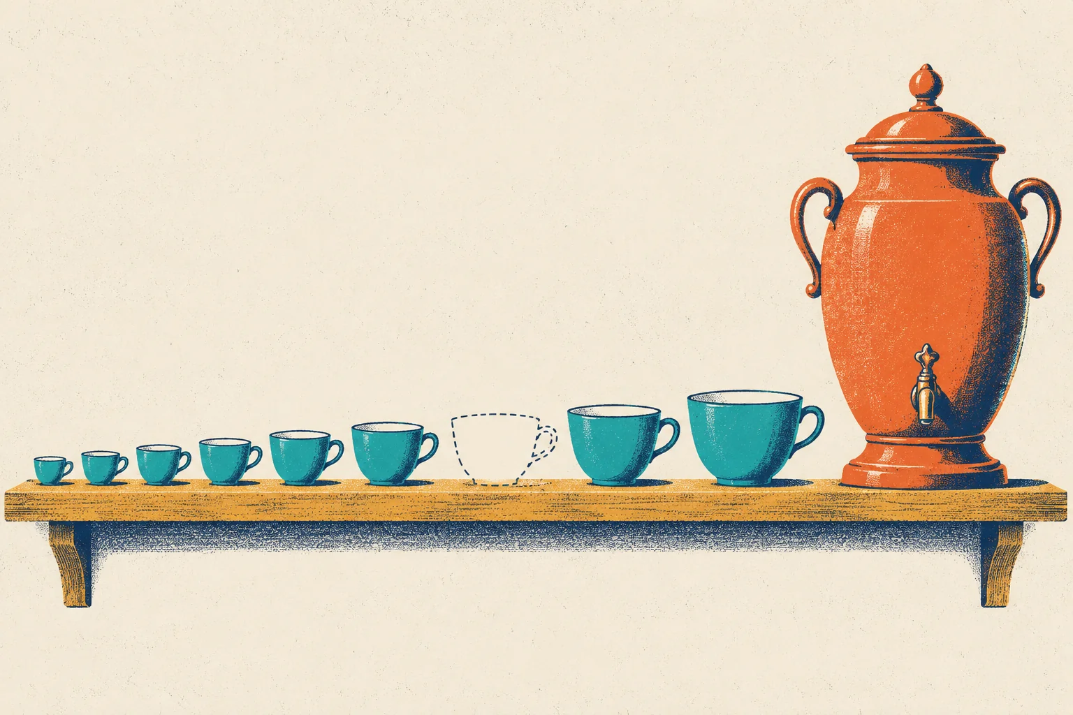
Look at the shelf in the picture. Most cups are small or middle-sized. At the far end stands one huge urn. In the middle of the row there is a dashed outline of a cup that nobody owns: the “average cup”. This chapter is about that outline. It shows where the average sits, but no real cup stands there. And the urn, one single object, pulls the average far more than any cup does.

Three ways to say “typical”

Imagine five orders at one counter: $8, $9, $9, $10, and $2,000 from an office that ordered tea for everyone.

The mean is what most people call “the average”. Add up all the values and divide by how many there are. Here, that is $2,036 ÷ 5 = $407.20. No order on the list is anywhere near $407.20.

The median is the middle value when you sort the values from smallest to largest. Half of the values are at or below it, and half are at or above it. Here, the median is $9. The office’s order does not move it. The median looks only at each value’s place in the sorted list, not at its size. If the office had spent $200,000, the median would still be $9.

There is a third way. The mode is the most common value: $9 here, because it appears twice.

None of these three is “the right average”. Each one answers a different question. The mean answers: if all the money were shared out equally, how much would each order get? The median answers: what does an order in the middle look like? To choose, you need to see the shape of all the values first.

The shape of Steep’s orders

Last week, Steep had 43,153 completed orders (final statuses, see Chapter 1). You cannot read 43,153 numbers, but you can sort them into groups and count each group.

A distribution is the full pattern of how often each value occurs. A histogram draws it: cut the range of values into equal pieces, called bins, and draw one bar per bin. The height of a bar is the number of values in that bin.

Show the code

fig, ax = bk.figure(8, 4.0)
ax.bar(edges[:-1], hist, width=0.5, align="edge", color=bk.TEAL, alpha=0.9)
top = hist.max()
ax.axvline(s2["median"], color=bk.INK, lw=2)
ax.axvline(s2["mean"], color=bk.TOMATO, lw=2, ls="--")
ax.text(s2["median"] - 0.3, top * 1.02, f"median {usd(s2['median'])}", ha="right", fontsize=10, color=bk.INK)
ax.text(s2["mean"] + 0.3, top * 1.02, f"mean {usd(s2['mean'])}", ha="left", fontsize=10, color=bk.TOMATO)
ax.text(HIST_MAX - 0.5, top * 0.5, f"{n(above_chart)} orders above ${HIST_MAX}\nare off the chart.\n"
        f"The largest: {usd(biggest.value)}", ha="right", fontsize=9.5, color=bk.INK)
ax.set_xlim(0, HIST_MAX)
ax.set_ylim(0, top * 1.12)
ax.xaxis.set_major_formatter(mticker.FuncFormatter(lambda v, _: f"${v:.0f}"))
ax.set_xlabel("Order value")
ax.set_ylabel("Orders")
ax.set_title("Steep's orders come in humps, and the mean falls between them")
plt.show()

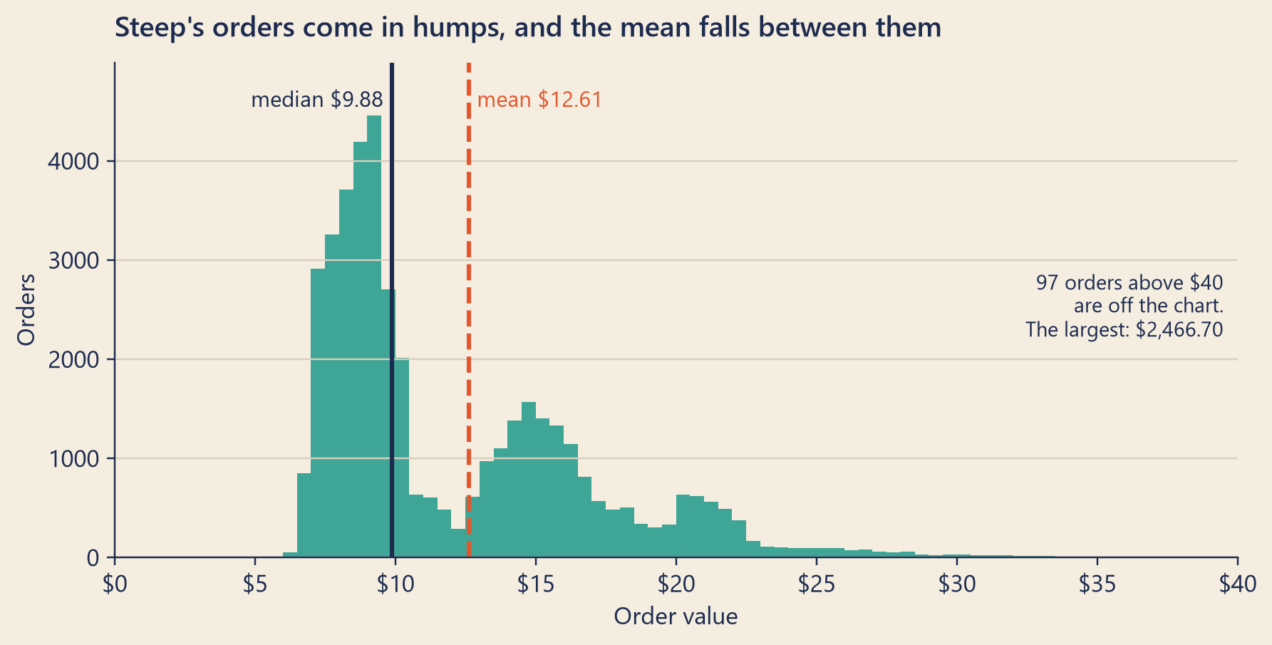
Histogram of order values from 0 to 40 dollars. A tall hump sits between about 7 and 10 dollars. A second, lower hump sits between about 13 and 16 dollars, and a small third one near 20 to 21 dollars. A solid navy line marks the median, near 10 dollars, inside the first hump. A dashed tomato line marks the mean, near 12.6 dollars, in the low gap between the first two humps. — Figure 1: Last week’s completed orders by value (what the customer paid), in bins of 50 cents. Orders above $40 are not drawn.

This is not the smooth hill that many people picture. It has humps. The tallest hump is the one-drink orders: 58% of all orders, most of them between $7.21 and $10.39, delivery fee included. The second hump is the two-drink orders: 29%, mostly between $11.99 and $17.85. Then come smaller humps for three drinks and more.

The median, $9.88, sits inside the big hump: it looks like a real order. The mean, $12.61, falls in the low gap between the first two humps. Only 2.5% of last week’s orders cost within 50 cents of the mean. That is the dashed cup in the picture: the “average order” is a place where hardly any order is.

Percentiles: a ruler for the shape

The median splits the orders in two halves. You can split them at other points too. A percentile is the value below which a given share of the values falls. The 90th percentile, written P90, is the value that 90% of orders are below. The median is the 50th percentile, P50.

Percentile	P10	P25	P50 (median)	P75	P90	P99	Largest
Last week	$7.72	$8.52	$9.88	$15.14	$19.73	$28.05	$2,466.70

Read the table from left to right, and it describes the shape in words. The middle half of the orders cost between $8.52 and $15.14. Nine orders in ten cost less than $19.73, and 99 in 100 less than $28.05. Then the last step, from P99 to the largest order, is far bigger than all the other steps together.

When you meet a new distribution, ask three questions. Where is the middle? The median answers that. How wide is the middle? The distance from P25 to P75 answers that. What is in the tails, the far ends of the distribution where the smallest and the largest values sit? For the large end, look at P90 and P99, and then at the largest values themselves, one by one.

The long tail

When a few values sit very far out on one side, the distribution has a long tail on that side. A distribution whose long tail points to the right, toward large values, is right-skewed. Skew is the word for this lopsided shape.

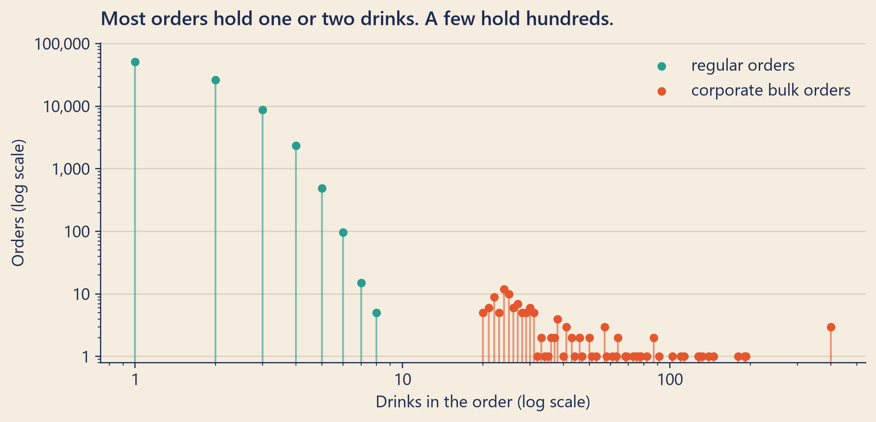
Steep’s long tail comes from one kind of customer. By that Tuesday, Steep had 84,654 registered users, and 236 of them were corporate accounts: companies that order tea for a whole office. They place bulk orders, from 20 up to 400 drinks at once, and only on weekdays. In the two weeks, they placed 140 orders. That is 0.16% of all orders, but 3.7% of all the money.

Show the code

counts = orders.groupby(["drinks", "corporate"]).size().reset_index(name="orders")
fig, ax = bk.figure(8, 3.8)
for is_corp, color, label in ((False, bk.TEAL, "regular orders"), (True, bk.TOMATO, "corporate bulk orders")):
    part = counts[counts.corporate == is_corp]
    ax.vlines(part.drinks, 0.8, part.orders, color=color, lw=1.2, alpha=0.6)
    ax.scatter(part.drinks, part.orders, color=color, s=22, zorder=3, label=label)
ax.set_xscale("log")
ax.set_yscale("log")
ax.set_ylim(0.8, counts.orders.max() * 2)
ax.xaxis.set_major_formatter(mticker.FuncFormatter(lambda v, _: f"{v:g}"))
ax.yaxis.set_major_formatter(mticker.FuncFormatter(lambda v, _: f"{v:,.0f}"))
ax.set_xlabel("Drinks in the order (log scale)")
ax.set_ylabel("Orders (log scale)")
ax.legend(loc="upper right")
ax.set_title("Most orders hold one or two drinks. A few hold hundreds.")
plt.show()

A chart on log scales. Orders with one drink number in the tens of thousands, and the counts fall fast for two, three and up to eight drinks. Then there is a gap. From 20 drinks to 400 drinks there are scattered points, each with one to about a dozen orders: the corporate bulk orders. — Figure 2: Completed orders in the two weeks by number of drinks. Both axes use a log scale: each step is ten times the one before.

The largest order of the two weeks had 400 drinks and cost $2,466.70. It is the urn on the shelf.

One order can move the mean

Here is what one urn does to one store. On Tuesday 8 September, Steep Harbor #6 had 332 completed orders. Of these, two were bulk orders, including that 400-drink one.

Steep Harbor #6, Tuesday 8 September	Mean	Median
Without the 2 bulk orders	$11.98	$9.59
With them	$19.84	$9.59

Two orders out of 332 raised the store’s mean by 66%. The median did not move at all.

A value far away from the rest is called an outlier. An outlier is not always a mistake. These bulk orders are real: a corporate account ordered hundreds of drinks and paid for them. The mean is honest about them. It includes every dollar. That is exactly why it moves.

How far one outlier moves the mean depends on how many other values share the load. In that store, on that day, the $2,466.70 order alone added about $7.42 to the mean. Among all 43,153 orders of the week, the same order adds about 6 cents. The smaller the group, the more one big value matters.

Back to Dana’s tile

Now Mia could read the tile. First, its definition. The tile uses the dashboard’s orders, keeps those still completed when the dashboard was last updated, and averages what they paid.

Chapter 1 said that the dashboard’s count ignores status. The tile cannot. An event does not say how much the customer paid, so the tile matches each event to its row in the orders table. That row also holds the order’s status, and the tile keeps only the completed ones.

Mia worked from the orders database itself, where every order is. Her charts, like every chart in this book, use final statuses (see Chapter 1). For this tile, that makes one difference. A corporate account’s order of 246 drinks from that Wednesday was refunded weeks later. With final statuses, the tile and the database tell much the same story.¹

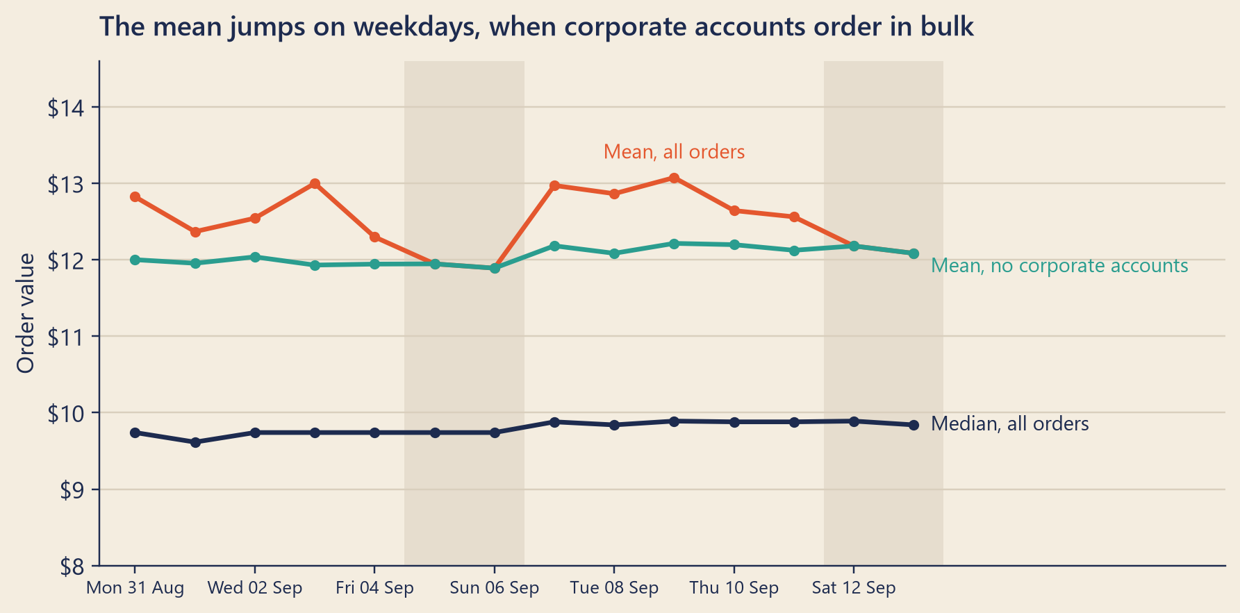
Mia drew the mean order value for each day of the two weeks. She drew it once with every order, once without the corporate accounts, and she added the median. In this chapter, regular customers means every customer who is not a corporate account.

Show the code

fig, ax = bk.figure(8, 3.9)
for day in daily.index[daily.index.dayofweek == 5]:
    ax.axvspan(day - pd.Timedelta(hours=12), day + pd.Timedelta(days=1, hours=12), color=bk.GRID, alpha=0.5, lw=0)
series = [("mean", bk.TOMATO), ("mean_regular", bk.TEAL), ("median", bk.INK)]
for column, color in series:
    ax.plot(daily.index, daily[column], color=color, lw=2.2, marker="o", ms=4)
# Label each line where it does not touch the others (on weekends the two means meet).
peak = daily["mean"].idxmax()
ax.annotate("Mean, all orders", (peak, daily.loc[peak, "mean"]), xytext=(0, 9),
            textcoords="offset points", ha="center", fontsize=9.5, color=bk.TOMATO)
ax.annotate("Mean, no corporate accounts", (daily.index[-1], daily["mean_regular"].iloc[-1]), xytext=(8, -2),
            textcoords="offset points", va="top", fontsize=9.5, color=bk.TEAL)
ax.annotate("Median, all orders", (daily.index[-1], daily["median"].iloc[-1]), xytext=(8, 0),
            textcoords="offset points", va="center", fontsize=9.5, color=bk.INK)
ax.set_xlim(daily.index[0] - pd.Timedelta(days=0.6), daily.index[-1] + pd.Timedelta(days=5.2))
ax.set_ylim(np.floor(daily["median"].min()) - 1, np.ceil(daily["mean"].max()) + 0.6)
ax.yaxis.set_major_formatter(mticker.FuncFormatter(lambda v, _: f"${v:.0f}"))
ax.set_xticks(daily.index[::2], [d.strftime("%a %d %b") for d in daily.index[::2]], fontsize=8.5)
ax.set_ylabel("Order value")
ax.set_title("The mean jumps on weekdays, when corporate accounts order in bulk")
plt.show()

Line chart over 14 days. The mean of all orders, in tomato, rises on weekdays and drops on each weekend. The mean without corporate accounts, in teal, is almost flat, close to 12 dollars. The median, in navy, is flat near 10 dollars in both weeks, slightly higher in the second week. — Figure 3: Mean and median order value by day, from the orders database. Grey bands mark the weekends, when corporate accounts do not order. The vertical axis does not start at zero.

The tile’s fall from Wednesday to Sunday was the long tail at work. On weekdays, corporate accounts place bulk orders: between 11 and 19 of them on each weekday of the two weeks. On weekends, there are none. So the mean of all orders rises on weekdays and drops every weekend. Without the corporate accounts, the mean went from $12.22 on that Wednesday to $12.09 on Sunday, a change of −1.1%. The median hardly moved in the two weeks.

So customers bought hardly less on Sunday. Corporate accounts do not order on Sundays.

To compare like with like, Mia put Sunday next to Sunday. The mean of all orders was $11.89 on 6 September and $12.09 on 13 September. Up, not down.

What to do with an outlier

You have four honest choices. Pick one before you look at the result, and say which one you picked.

Use the median, or report percentiles, when the question is about a typical order.
Use a trimmed mean. A trimmed mean drops a fixed share of the smallest and the largest values, and takes the mean of the rest. A 5% trimmed mean drops the lowest 5% and the highest 5%. Last week’s 5% trimmed mean was $11.75, between the median and the mean.
Split the data. Report regular customers and corporate accounts as two segments. A segment is a group of customers or orders that you look at separately. These two are different kinds of customer, and each one has a calmer shape on its own.
Cap the values. Replace every value above a limit with the limit. Chapter 21 uses this method, called winsorizing, in an A/B test.

One choice is not honest: deleting outliers because they make the result look bad. If you choose what to remove after you see which way it pushes, you will push the answer toward the one you hoped for.

When the mean is the right number

After all this, you might think that the median always wins. It does not.

Suppose finance wants to plan next week’s cash. They need total revenue, and total revenue is the number of orders times the mean order value. This works only with the mean. Try it with the median for the week before: 45,441 orders × $9.74 = $442,595. The real total was $563,367. The median misses $120,771, 21% of the money, because it ignores how big the big orders are.

So the rule is not “median good, mean bad”. If you will add up or multiply the number, use the mean, with every value in it. If you want to describe a typical case, use the median or percentiles. Many reports should show both, with the number of values.

The median can be too calm

The median has a blind spot of its own. Steep sells a dozen drinks at fixed prices, so thousands of orders cost exactly the same amount. The median sits on one of these common prices and jumps from one to the next. In the week before, the daily median was exactly $9.74 on six of the seven days.

It also ignores everything far from the middle. Every order with three drinks or more costs more than the median. If all of those orders had cost $5 more, the median would not have moved by one cent.

The mode is even more fragile. The most common order value was $7.74 in the week before and $7.24 last week, while the median went up. With so many prices close together, the top spot can change hands from one week to the next.

So no single number is enough. Use the median for the middle, percentiles for the spread, and the mean, with its count, for totals.

Did customers buy less each time?

Now Mia could answer Dana’s question. She put the two weeks side by side.

Completed orders	The week before	Last week	Change
Number of orders	45,441	43,153	−5.0%
Median order value	$9.74	$9.88	+1.4%
Mean order value	$12.40	$12.61	+1.7%
Mean, no corporate accounts	$11.96	$12.15	+1.6%
5% trimmed mean	$11.56	$11.75	+1.6%
P90	$19.59	$19.73	+0.7%
Median drinks per order	1	1	no change
Mean drinks per order	1.70	1.65	−3.0%
Revenue	$563,367	$544,154	−3.4%

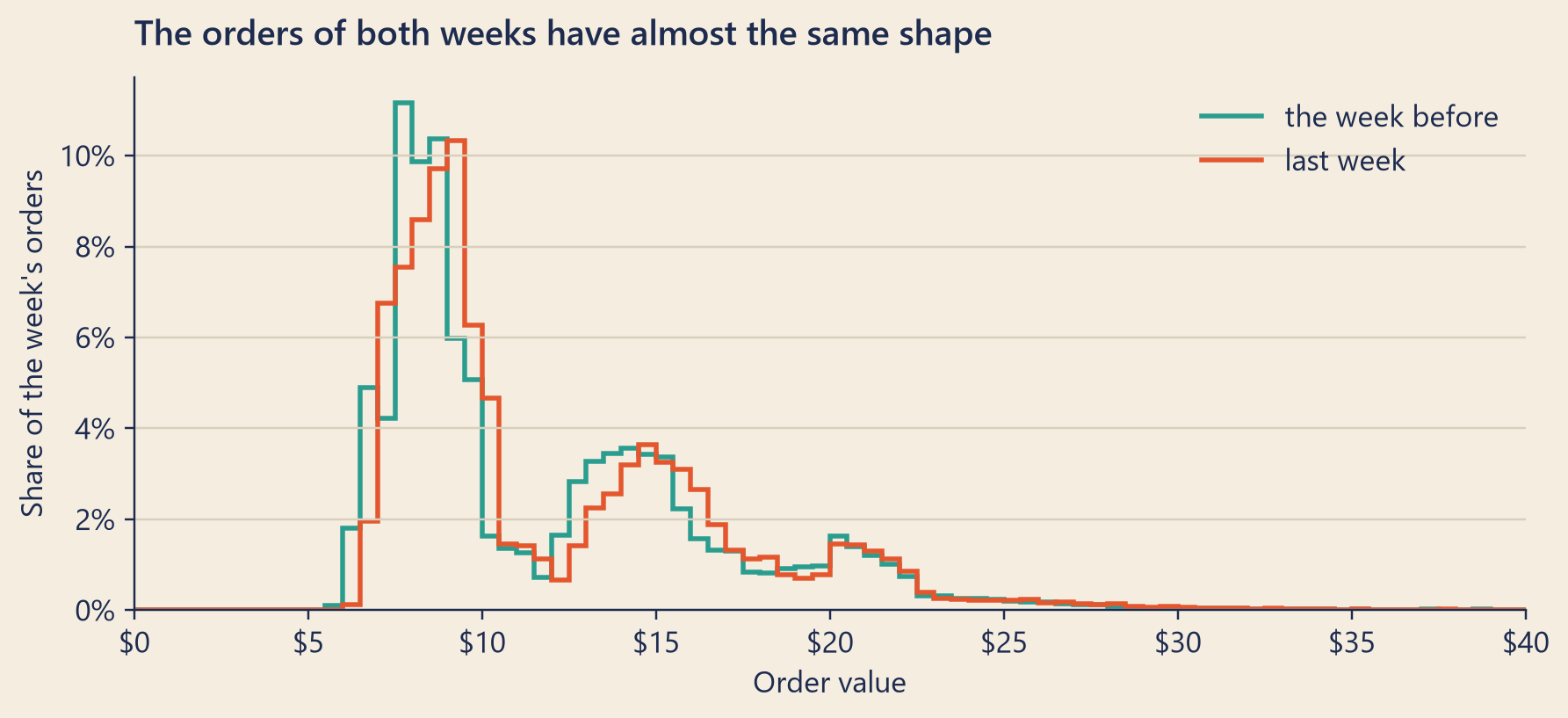
Every measure of order value went up a little, not down. The median order rose from $9.74 to $9.88.

Show the code

fig, ax = bk.figure(8, 3.6)
for frame, label, color in ((w1, "the week before", bk.TEAL), (w2, "last week", bk.TOMATO)):
    share, _ = np.histogram(frame.value, bins=edges)
    ax.stairs(share / len(frame), edges, color=color, lw=1.8, label=label)
ax.set_xlim(0, HIST_MAX)
ax.xaxis.set_major_formatter(mticker.FuncFormatter(lambda v, _: f"${v:.0f}"))
ax.yaxis.set_major_formatter(mticker.PercentFormatter(1.0, decimals=0))
ax.set_xlabel("Order value")
ax.set_ylabel("Share of the week's orders")
ax.legend(loc="upper right")
ax.set_title("The orders of both weeks have almost the same shape")
plt.show()

Two step lines, teal for the week before and tomato for last week, almost on top of each other. Both show the same humps at the same places. The tomato line sits slightly to the right. — Figure 4: Share of each week’s completed orders in each 50-cent bin. Orders above $40 are not drawn.

The shape of an order hardly changed. Last week’s line sits a little to the right: across the middle of the distribution, the percentiles (P10, P25, the median and P75) rose by 14 to 30 cents. The count of orders is what changed. Revenue is the count times the mean: the count fell 5.0%, the mean rose 1.7%, and 0.950 × 1.017 ≈ 0.966. So revenue from completed orders fell 3.4%, less than the count.

Mia saw one more small thing. Drinks per order fell from 1.70 to 1.65, about 3%. Fewer orders and fewer drinks in each order: together they explain why drinks fell faster than orders in Chapter 1 (0.950 × 0.970 ≈ 0.921, a fall of 7.9%). Regular customers alone show almost the same fall in drinks per order, −2.9%, so it is not the bulk orders. Yet the money per order went up. This is about the size of each order, so it cannot explain why there were fewer orders. She did not have an explanation for it, so she wrote it down as a question, not a clue: Fewer drinks per order, but more money per order. Why? Chapter 21 returns to this.

Under the hood

Mean and median. For values $x_1, \dots, x_n$, the mean is $\bar{x} = \frac{1}{n}\sum_{i=1}^{n} x_i$. Sort the values: $x_{(1)} \le x_{(2)} \le \dots \le x_{(n)}$. The median is $x_{((n+1)/2)}$ when $n$ is odd, and the mean of the two middle values when $n$ is even.

One new value. Add one value $v$ to $n$ values with mean $\bar{x}$. The new mean is

\[\bar{x}' = \frac{n\bar{x} + v}{n + 1} = \bar{x} + \frac{v - \bar{x}}{n + 1}.\]

The shift is the distance of the new value from the mean, divided by $n + 1$. That is why the same order moves a store’s daily mean by dollars and a week’s mean by cents. The median moves at most to the next value in the sorted list, however large $v$ is.

Robustness. The breakdown point of a statistic is the share of values you would have to replace with wild values to move it as far as you like. For the mean, one value is enough, so as $n$ grows the breakdown point goes to 0%. For the median it is 50%. A trimmed mean that drops 5% at each end has a breakdown point of 5%.

Trimmed mean. With $k = \lfloor \alpha n \rfloor$ (here $\alpha = 0.05$), drop the $k$ smallest and the $k$ largest values, and take the mean of the other $n - 2k$.

Percentiles. There are several conventions for values that fall between two data points. pandas, NumPy and DuckDB’s quantile_cont draw a straight line between the two neighbours. DuckDB’s quantile_disc returns an actual value from the data instead. With many repeated values, as here, they usually agree.

Skew. One common measure is the sample skewness, $\frac{1}{n}\sum (x_i - \bar{x})^3 / s^3$, where $s$ is the standard deviation, a common measure of how spread out the values are. Last week’s order values have a skewness of 78. Remove the one largest order and it falls to 34. Like the mean, skewness is pushed by a few huge values. Without the corporate accounts, it is 1.3. A symmetric shape has 0. Textbooks often say “in right-skewed data, the mean is above the median”. That is common, but it is not a law: von Hippel (2005) shows real cases that break it. Look at the data instead of trusting the rule.

Try it

Drag an outlier. The bars are real orders from regular customers. Add bulk orders and watch the three averages. Each bulk drink costs $5.78, the average for bulk orders in these two weeks. Teal shows the values before you add anything; tomato shows them after.

Show the code

viewof outSample = Inputs.radio(
  new Map(outFacts.samples.map(s => [s.label, s.id])),
  {value: "store", label: "Orders"})
viewof outCount = Inputs.range([0, 3], {value: 1, step: 1, label: "Bulk orders to add"})
viewof outDrinks = Inputs.range([outFacts.bulkMin, outFacts.bulkMax],
  {value: outFacts.bulkMax, step: 10, label: "Drinks in each bulk order"})

Show the code

// Mean, median and trimmed mean of [value, count] pairs sorted by value.
function summarize(pairs, trim) {
  let n = 0, sum = 0;
  for (const [v, c] of pairs) { n += c; sum += v * c; }
  const at = k => {  // the k-th smallest value, counting from 0
    let seen = 0;
    for (const [v, c] of pairs) { seen += c; if (k < seen) return v; }
    return pairs[pairs.length - 1][0];
  };
  const median = n % 2 ? at((n - 1) / 2) : (at(n / 2 - 1) + at(n / 2)) / 2;
  const cut = Math.floor(trim * n);
  let kept = 0, index = 0;
  for (const [v, c] of pairs) {
    const lo = Math.max(index, cut), hi = Math.min(index + c, n - cut);
    if (hi > lo) kept += v * (hi - lo);
    index += c;
  }
  return {n, mean: sum / n, median, trimmed: kept / (n - 2 * cut)};
}

Show the code

outView = {
  const C = {teal: "#2a9d8f", tomato: "#e4572e", tomatoText: "#b8401c", ink: "#1d2b4f", muted: "#8a8f9e"};
  const sample = outFacts.samples.find(s => s.id === outSample);
  const bulkValue = Math.round(outDrinks * outFacts.perDrink * 100) / 100;
  const before = summarize(sample.pairs, outFacts.trim);
  const withBulk = outCount > 0 ? [...sample.pairs, [bulkValue, outCount]] : sample.pairs;
  const after = summarize(withBulk, outFacts.trim);

  const xMax = outFacts.xMax;
  const bins = Array.from({length: xMax}, (_, i) => ({x1: i, x2: i + 1, orders: 0}));
  for (const [v, c] of sample.pairs) bins[Math.min(xMax - 1, Math.floor(v))].orders += c;
  const tallest = Math.max(...bins.map(b => b.orders));
  const bulkX = xMax + 3;
  const money = x => "$" + x.toLocaleString("en-US", {minimumFractionDigits: 2, maximumFractionDigits: 2});
  const box = (document.querySelector("main") || document.body).clientWidth;
  const plotWidth = Math.max(300, Math.min(680, box - 40));
  const showAt = x => Math.min(x, bulkX - 1.5);  // a mean beyond the axis is drawn at its right edge

  const marks = [
    Plot.rectY(bins, {x1: "x1", x2: "x2", y: "orders", fill: C.teal, fillOpacity: 0.85, inset: 0.4}),
    Plot.ruleY([0], {stroke: C.ink}),
    Plot.ruleX([before.mean], {stroke: C.teal, strokeWidth: 2, strokeDasharray: "5,3"}),
    Plot.ruleX([showAt(after.mean)], {stroke: C.tomato, strokeWidth: 2.5}),
    Plot.ruleX([after.median], {stroke: C.ink, strokeWidth: 2}),
    Plot.text([{x: after.median, y: tallest * 1.13, t: "median"}], {x: "x", y: "y", text: "t", textAnchor: "end", dx: -4, fill: C.ink, fontSize: 11}),
    Plot.text([{x: showAt(after.mean), y: tallest * 1.13, t: outCount > 0 ? "mean, with bulk" : "mean"}], {x: "x", y: "y", text: "t", textAnchor: "start", dx: 4, fill: C.tomatoText, fontSize: 11})
  ];
  if (outCount > 0) {
    marks.push(Plot.rectY([{x1: bulkX - 1, x2: bulkX + 1, orders: outCount}], {x1: "x1", x2: "x2", y: "orders", fill: C.tomato}));
    marks.push(Plot.text([{x: bulkX, y: Math.max(outCount, tallest * 0.08)}],
      {x: "x", y: "y", text: () => `${outCount} × ${money(bulkValue)}`, dy: -10, fill: C.tomatoText, fontSize: 11, textAnchor: "end"}));
  }
  const plot = Plot.plot({
    width: plotWidth, height: 260, marginLeft: 48, marginRight: 12,
    style: {background: "transparent", fontSize: "11px", fontFamily: "Inter, system-ui, sans-serif"},
    x: {domain: [0, bulkX + 1.5], label: "Order value →", ticks: [0, 10, 20, 30, 40].filter(t => t <= xMax),
        tickFormat: d => "$" + d},
    y: {domain: [0, tallest * 1.2], label: "↑ Orders", grid: true},
    marks
  });

  const row = (label, a, b) => {
    const change = b / a - 1;
    const text = (change >= 0 ? "+" : "−") + Math.abs(100 * change).toFixed(1) + "%";
    return html`<tr><td>${label}</td><td class="num" style="color:${C.teal}">${money(a)}</td>
      <td class="num" style="color:${C.tomatoText}"><strong>${money(b)}</strong>
        <span class="out-change">${text}</span></td></tr>`;
  };
  return html`<div class="out-wrap">
    <style>
      .out-wrap { font-family: Inter, system-ui, sans-serif; color: ${C.ink}; }
      .out-wrap table.out-table { display: table; width: 100%; max-width: 30rem; border-collapse: collapse; font-size: 0.85rem; margin-top: 0.4rem; }
      .out-table th, .out-table td { padding: 0.25rem 0.4rem; border-bottom: 1px solid rgba(29,43,79,0.12); vertical-align: top; }
      .out-table .num { text-align: right; white-space: nowrap; }
      .out-change { display: block; font-size: 0.75rem; color: #3d4766; }
      .out-note { font-size: 0.85rem; color: #3d4766; margin: 0.3rem 0 0; }
    </style>
    ${plot}
    <p class="out-note">${before.n.toLocaleString("en-US")} regular orders ${outCount > 0
      ? html`+ <strong>${outCount}</strong> bulk order${outCount > 1 ? "s" : ""} of ${outDrinks} drinks
        (${money(bulkValue)} each), drawn at the far right, off the scale`
      : "and no bulk orders"}.</p>
    <table class="out-table">
      <thead><tr><th></th><th class="num">Before</th><th class="num">After (change)</th></tr></thead>
      <tbody>
        ${row("Mean", before.mean, after.mean)}
        ${row("Median", before.median, after.median)}
        ${row("5% trimmed mean", before.trimmed, after.trimmed)}
      </tbody>
    </table>
  </div>`;
}

Things to try:

With one store’s day, add one bulk order of 400 drinks. The mean jumps; the median does not move.
Keep the bulk order and switch to “All of Steep, last week”. The same order now moves the mean by cents.
Add three bulk orders to one store’s day. The trimmed mean starts to move too, but much less than the mean.
Set the drinks to 20. Even a small bulk order is far out in the tail of one store’s day.

Common traps

Reporting a mean without the shape. Before you write “the average order is $X”, look at the histogram and the percentiles, and say how many orders the mean covers.
Reading a moving mean as a change in customers. Dana’s tile moved because of who ordered on each day (corporate accounts on weekdays), not because customers changed. Compare like with like: weekdays with weekdays, and regular customers with regular customers.
Using the median to add things up. Totals, budgets and forecasts need the mean.
Deleting outliers after you see the result. Decide the rule first: median, trimmed mean, split, or cap.
Averaging averages. The mean of four city averages is not Steep’s average, unless every city has the same number of orders. Weight each average by its count, or go back to the orders.
Designing for “the average customer”. A product built for the person who orders 1.65 drinks fits nobody. Look at the humps: one-drink customers and corporate accounts need different things.

Audit Instinct · Test the big items, sample the rest

An auditor checking a year of invoices does not pick a random handful and hope. She looks at the shape first. Then she uses stratified sampling: she splits the population into layers, called strata, by size. She tests every item in the top layer, the few invoices that carry most of the money. Then she takes a random sample from the many small ones. A random sample of the whole list would usually miss the few large items, and they are where the money is.

Steep’s orders have the same shape. Last week, 76 bulk orders (0.18% of all orders) carried 3.8% of the money. The data version of the audit habit is this: list the largest values and look at each one, then describe the rest with medians and percentiles. Never let a single average speak for both layers.

Interview Corner

Q1. Mean or median for average order value? Why?

A short answer

It depends on the question. To describe a typical order, use the median and a few percentiles, because order values are right-skewed and a few large orders pull the mean. To plan revenue or cash, use the mean: only the mean times the number of orders gives the total. In practice, report both with the count, and show large customers (such as corporate accounts) as a separate segment.

Q2. How do you treat outliers in a KPI (key performance indicator: a number a team is judged by)?

A short answer

First find out whether they are errors or real. Fix errors at the source. For real values, choose a rule before you look at the result, write it down, and apply it every time. You can report a robust number (median, trimmed mean). You can split the outliers into their own segment. Or you can cap values at a percentile taken from past data. Never remove outliers after you see which way they push. Keep a list of the largest values, and look at it whenever the KPI moves.

Q3. Average order value fell 10% from Wednesday to Sunday. What do you check?

A short answer

First check the tile’s definition: what it averages, from which source, and with statuses as of when. Then check whether the same mix of orders is being compared. Look at the distribution for both days, the median and the top percentiles, and split by customer type and by weekday. A fall that disappears in the median, or in the regular customers, comes from the tail (here, weekday bulk orders), not from a change in typical customers. Then compare Sunday with earlier Sundays, not with a Wednesday.

Mia sent Dana a short message before lunch: “Orders did not get cheaper. The median order went up 14 cents. Your tile falls every weekend because corporate accounts do not order on weekends. What fell is the number of orders: about 5% in the database, 12% on the dashboard.”

Dana replied with one word: “Good.” Then a second message: “So where are the other 7 points?”

Reported change: −12.0% orders, the week of 7 September compared with the week before (CEO dashboard).

Explained so far: 0 of the 12 points.

Suspects: measurement (not proved). Clue 1: about 7 points live between the orders database and the dashboard (Chapter 1).

Ruled out: the choice of status, clock, week start or customers (Chapter 1). Smaller orders as the reason the count fell: order value did not fall (this chapter).

Open questions: Which orders have no order_completed event in the warehouse, and since when? Is the database’s fall of about 5% a fair comparison? Why did drinks per order fall about 3% while money per order rose? (Chapter 21 returns to this.)

New evidence: in the database, completed orders fell 5.0% (final statuses). The median order went from $9.74 to $9.88, and the mean from $12.40 to $12.61. What fell is the count of orders.

Recap

An average is one number for many values. Look at the distribution, its humps and its tail, before you trust it.
The median and percentiles describe a typical value and resist outliers. The mean adds up to the total, so use it for money you will add up or multiply.
An outlier can be real. Choose a rule for it before you see the result: median, trimmed mean, separate segment, or cap.

English	中文
mean	均值
median	中位数
mode	众数
percentile	分位数 / 百分位数
distribution	分布
histogram	直方图
long tail	长尾
skew	偏态
outlier	异常值
trimmed mean	截尾均值
breakdown point	崩溃点
tails	尾部
segment	细分群体
KPI (key performance indicator)	关键绩效指标
stratified sampling	分层抽样

Three ways to say “typical”

The shape of Steep’s orders

Percentiles: a ruler for the shape

The long tail

One order can move the mean

Back to Dana’s tile

What to do with an outlier

When the mean is the right number

The median can be too calm

Did customers buy less each time?

Try it

Common traps

Recap

Further reading