On Thursday morning, Priya Nair was waiting at Mia’s desk. She held her laptop against her chest, the way people hold a letter with bad news.
“Do you have ten minutes?” she asked. “I did not sleep well.”
Priya was Steep’s product manager. Her biggest project that summer was the matcha menu: a new menu page that puts matcha drinks first. On 3 August, seven of Steep’s 18 stores switched to it. The other stores kept the classic menu. On Monday, Priya had blamed the weather. By Thursday, she had started to worry about her own project.
She opened a chart from her product dashboard. It had two bars.
“Conversion since the launch,” she said. “Stores with the matcha menu: 24.9%. Stores with the classic menu: 27.1%. The matcha stores are worse. And now Dana says orders fell twelve percent.” She looked at the screen, not at Mia. “What if it is my menu? What if people open the matcha page, get confused, and leave?”
Mia opened her notebook. Monday had reminded her of an old audit habit: ask how a number is counted before you believe it. “What does ‘conversion’ count here?”
“Orders, divided by store visits. Each time someone in the app opens one store’s menu page, that is one store visit.”
“And where are the seven stores?”
“Four in Harbor, and one in each of the other three cities. Harbor is our biggest city. I wanted as many people as possible to see the new menu.”
Mia wrote the matcha menu? on her list of suspects. Then she drew a small table with four rows, one for each city. “Let’s not compare matcha stores with classic stores,” she said. “Let’s compare them inside each city.”
Twenty minutes later, the table was full. In every city, the matcha stores converted better than the classic stores. Priya read the table three times.
“Better in every city,” she said slowly, “and worse in total? How is that possible?”
“It is a famous puzzle,” said Mia. “It has a name. And I think it is going to clear your menu.”
ImportantThe big idea
A trend that holds in every group can reverse when you add the groups together, if the two things you compare are spread over the groups very differently.
Look at the picture above. On the shelf stand four small scales, one for each city. Each pan holds one tea tin, and every small scale sinks a little on its teal side. Above them, a large scale holds more tins: three in the teal pan and six in the tomato pan. It sinks on the tomato side.
In this chapter, teal is the classic menu and tomato is the matcha menu. On these scales, the lower pan is the loser: the side that converts worse. In each city, classic sinks. In total, matcha sinks, because its pan is loaded differently: most of its weight comes from one place. By the end of the chapter, you will know which place, and why that is enough to tip the scale.
Priya’s number
A conversion rate is the share of chances that end in the thing you want. A shop might count the share of people who walk in and buy something. A session is one visit to the app, from opening it to leaving it. Priya’s chances are store visits: one session that opens one store’s menu page. One session can visit several stores. A customer may look at three stores and order from one. The thing she wants is an order. So her conversion rate is orders divided by store visits.
The app’s events do not say which store’s page a customer opened. The store-menu service keeps its own log of store visits. Mia added up the log herself, for the six weeks from the launch on 3 August to 13 September:
Menu
Stores
Store visits
Orders
Conversion
Classic
11
566,409
153,222
27.1%
Matcha
7
481,890
120,061
24.9%
Priya’s numbers were right. The matcha stores converted 2.1 percentage points worse: 24.91% against 27.05%. (A percentage point is one step on the percent scale: from 27% to 25% is two points.) The question was what the gap meant.
Split it by city
A segment is a part of the data that shares one feature, such as a city, a platform or a menu. Segmenting means splitting the data into segments and comparing inside each one. It is one of the oldest tricks in analysis, and you have already used it: in Chapter 3, splitting the orders by platform showed that the dashboard’s gap sits on iOS.
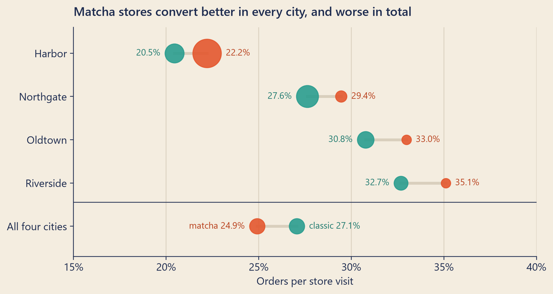
Mia split the store visits by city. Here is what she found.
Show the code
fig, ax = bk.figure(8, 4.2)rows = CITIES + ["all"]ypos = {c: len(rows) -1- i for i, c inenumerate(rows)}scale =900/ visits.values.max() # marker area in points², by visitsdef dot(x, y, area, color, label, label_color, side):"""One dot, with its label just outside the dot on the given side (-1 left, +1 right).""" ax.scatter(x, y, s=area, color=color, zorder=3, alpha=0.9) gap_pt = np.sqrt(area) /2+5 ax.annotate(label, (x, y), xytext=(side * gap_pt, 0), textcoords="offset points", ha="left"if side >0else"right", va="center", fontsize=9.5, color=label_color)for c in CITIES: y = ypos[c] ax.plot([conv.classic[c], conv.matcha[c]], [y, y], color=bk.GRID, lw=3, zorder=1) k_side =-1if conv.classic[c] < conv.matcha[c] else1 dot(conv.classic[c], y, visits.classic[c] * scale, bk.TEAL, rate(conv.classic[c]), TEAL_TEXT, k_side) dot(conv.matcha[c], y, visits.matcha[c] * scale, bk.TOMATO, rate(conv.matcha[c]), TOMATO_TEXT, -k_side)y = ypos["all"]ax.axhline(y +0.55, color=bk.INK, lw=0.8)ax.plot([total_m, total_k], [y, y], color=bk.GRID, lw=3, zorder=1)dot(total_k, y, 260, bk.TEAL, f"classic {rate(total_k)}", TEAL_TEXT, 1if total_k > total_m else-1)dot(total_m, y, 260, bk.TOMATO, f"matcha {rate(total_m)}", TOMATO_TEXT, 1if total_m > total_k else-1)ax.set_yticks([ypos[c] for c in rows], [CITY.get(c, "All four cities") for c in rows])ax.set_xlim(0.15, 0.40)ax.set_ylim(-0.7, len(rows) -0.4)ax.xaxis.set_major_formatter(lambda v, _: f"{v:.0%}")ax.grid(axis="y", visible=False)ax.grid(axis="x", color=bk.GRID)ax.set_xlabel("Orders per store visit")ax.set_title("Matcha stores convert better in every city, and worse in total")plt.show()
Figure 1: Conversion (orders per store visit), 3 August to 13 September. Each dot’s area shows how many store visits it stands for. The bottom row adds the four cities together.
In Harbor, the matcha stores converted 22.2% of their visits, and the classic stores 20.5%. In Northgate, 29.4% against 27.6%. In Oldtown, 33.0% against 30.8%. In Riverside, 35.1% against 32.7%. In every city, matcha was ahead, by between 1.8 and 2.4 points. Add the cities together, and matcha is behind.
This is called Simpson’s paradox: a comparison that holds inside every group reverses when you combine the groups. It is named after Edward Simpson, a British statistician who wrote about it in 1951, although others had noticed it before him. It is not really a paradox. Nothing in the data is wrong. It only feels wrong, because we expect a total to agree with its parts.
Where the weight sits
Look at the size of the dots again. The big tomato dot is in Harbor. The teal dots are spread more evenly. This is the whole secret.
Every total rate is a weighted average of its segments: an average in which each part counts in proportion to its size. Tea makes this easy to picture. Pour three cups of strong tea and one cup of weak tea into a pot. The pot tastes strong, because most of it came from the strong cups. The pot’s taste is a weighted average of the cups.
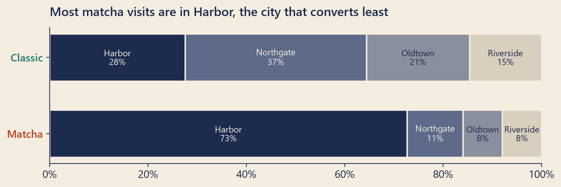
The mix of a total is how it is split between the segments. Here are the two mixes:
Show the code
order =list(city_conv.sort_values().index)shades = {"harbor": bk.INK, "northgate": "#5d6a89", "oldtown": bk.MUTED, "riverside": bk.GRID}fig, ax = bk.figure(8, 2.6)for y, menu in [(1, "classic"), (0, "matcha")]: left =0.0for c in order: share = mix[menu][c] ax.barh(y, share, left=left, color=shades[c], height=0.62, edgecolor=bk.PAPER, lw=1.5)if share >0.07: dark = c in ("harbor", "northgate") ax.text(left + share /2, y, f"{CITY[c]}\n{rate(share, 0)}", ha="center", va="center", fontsize=9, color=bk.PAPER if dark else bk.INK, linespacing=1.1) left += shareax.set_yticks([1, 0], ["Classic", "Matcha"])for label, color inzip(ax.get_yticklabels(), (TEAL_TEXT, TOMATO_TEXT)): label.set_color(color) label.set_fontweight("semibold")ax.set_xlim(0, 1)ax.xaxis.set_major_formatter(lambda v, _: f"{v:.0%}")ax.grid(False)ax.set_title("Most matcha visits are in Harbor, the city that converts least")plt.show()
Figure 2: Where each menu’s store visits happened, 3 August to 13 September. The cities are in order of conversion, from lowest (Harbor) to highest (Riverside).
73% of the matcha stores’ visits happened in Harbor. For the classic stores, it was only 28%. And Harbor converts less than any other city: 21.7% of its store visits end in an order, against 33.4% in Riverside.
So the matcha total is mostly a Harbor number. Here is the weighted average, written out. Each city’s share of the matcha visits is multiplied by the matcha rate in that city, and the four results are added up:
City
Share of matcha visits
Matcha conversion
Share × conversion
Harbor
72.7%
22.2%
16.14%
Northgate
11.4%
29.4%
3.35%
Oldtown
8.0%
33.0%
2.64%
Riverside
7.9%
35.1%
2.79%
Matcha total
100%
24.91%
(Each part is rounded, so the parts may miss the total by a hundredth of a point.)
Each matcha store beats its neighbours. But matcha’s pot is filled mostly from Harbor’s cups, and Harbor’s cups are weak. The classic pot gets more of its tea from the strong cups of the smaller cities. A difference in totals that comes from a difference in the mix is called a mix shift or a composition effect. Inside each city, nothing is worse. Only the weights are different.
Why Harbor converts least
Mia did not stop there. A city with a low conversion rate is itself a number to question. Do people in Harbor really order less?
They do not. Mia counted shopping sessions: app sessions in which a customer opened the menu. In every city, between 43.5% and 43.9% of them ended in an order. The difference is in the store pages. Harbor has the most stores, and a Harbor customer opened 2.0 store pages per session, on average. In the other cities, it was between 1.3 and 1.6. More pages for the same orders means more store visits, so a lower rate per visit.
This is Chapter 1’s lesson again: a number is a definition. “Orders per store visit” punishes a city where people like to look around.
A third thing behind both
Why did the menu and the city get tangled up? Because of a choice. Priya put four of her seven stores in Harbor, because Harbor is the biggest city. So the city decided which stores got matcha. And the city also decides the conversion rate, because of all those store pages.
A confounder is a third thing that affects both the groups you compare and the result you measure. Here, the city is a confounder. It pushed matcha into Harbor, and it pushed Harbor’s rate down. When a confounder is at work, a plain comparison of totals mixes up two stories: the effect of the menu and the effect of the place. Splitting by the confounder pulls the two stories apart.
The same stores, before the matcha menu
Mia had one more test in mind. It is a simple and strong one. Before 3 August, the seven stores had the classic menu, like every other store. If the gap comes from the places and not from the menu, those stores should have looked “worse” in total before they had matcha.
She took the six weeks before the launch, from 22 June to 2 August:
City
The seven stores, before
The other stores, before
Matcha, after
Classic, after
Harbor
21.8%
21.9%
22.2%
20.5%
Northgate
28.0%
28.1%
29.4%
27.6%
Oldtown
31.7%
31.3%
33.0%
30.8%
Riverside
33.8%
33.7%
35.1%
32.7%
All four cities
24.3%
28.0%
24.9%
27.1%
Before the launch, with no matcha menu anywhere, the same seven stores converted 24.3% in total, against 28.0% for the others. They “lost” by even more than after the launch. Inside each city, they were level with their neighbours: never more than 0.3 points apart.
So the gap in Priya’s chart belongs to the places, not to the menu. It was there before matcha existed.
Back to the case
Priya’s real fear was not about conversion. It was about the twelve percent. Could the matcha menu explain the fall from the week before (31 August to 6 September) to last week (7 to 13 September)?
Mia thought about the timing first. The matcha menu started on 3 August, five weeks before the drop. It was at the same seven stores in both weeks. A thing that did not change between two weeks cannot, on its own, explain a change between them.
Then she checked the orders in the database, store by store. From the week before to last week, orders at the matcha stores changed by −4.4%. At the classic stores, they changed by −5.2%. The matcha stores did not lose more orders than the others.
Mia crossed out the matcha menu? in her notebook and wrote next to it: not a suspect.
Priya let out a long breath. Then she smiled. “So matcha raises conversion. Two points in every city!”
“Not so fast,” said Mia.
Does matcha make people order more?
The city table shows that the matcha stores converted better than their neighbours. It does not show that the matcha menu caused it. Mia gave four reasons.
The stores were chosen, not drawn at random. Priya picked them. Perhaps she picked stores that were already improving, or stores with a very good manager. The test before the launch helps here: inside each city, the seven stores were level with their neighbours before matcha. That is a good sign, but it is a hint, not proof.
A rate has two parts: orders on top, visits below. From the six weeks before the launch to the six weeks after, orders at the seven stores changed by +1.1%, and at the other stores by +0.7%. Store visits changed by −1.3% at the matcha stores. So the matcha stores’ rate rose from 24.3% to 24.9% for two reasons of about the same size: a few more orders, and a few fewer visits. Fewer people browsed a matcha page and left. Whether that is good for Steep is a separate question.
The neighbours changed too. A shopper who skips a matcha page often opens a classic page instead. After the launch, the classic stores got 4% more visits, and they converted less in every city:
City
The seven stores, before
Matcha, after
Classic stores, before
Classic, after
Harbor
21.8%
22.2%
21.9%
20.5%
Northgate
28.0%
29.4%
28.1%
27.6%
Oldtown
31.7%
33.0%
31.3%
30.8%
Riverside
33.8%
35.1%
33.7%
32.7%
Look at Harbor. Matcha stores rose 0.4 points; classic stores fell 1.4. So part of matcha’s lead is its neighbours getting worse. The neighbours are not an untouched comparison.
Other things change too. Weather, prices, a new store nearby: anything that hit some stores and not others can hide inside a before-and-after comparison.
The surest way to know whether the matcha menu causes more orders is a random choice of who gets it. Because shoppers move between stores, Steep should choose customers at random, not stores: each customer then sees one menu at every store. That is an experiment, and Part IV is about how to run one.
“So it is innocent,” said Priya, “but not a hero.”
“Innocent of the drop,” said Mia. “We don’t know yet about the hero part.”
When to split, and when splitting fools you
Simpson’s paradox does not mean “always split” or “never trust a total”. It means you must know why you split. Three rules help.
Split by something that was fixed before the change. The city of a store did not change because of the menu. It came first. That makes it safe to split by. Now imagine splitting by “sessions that opened three or more store pages”. The menu itself could change how many pages people open. If you split by something the change can affect, the split can show a gap the change did not cause, or hide one it did.
Both numbers can be true. They answer different questions. “Is the matcha menu worse than the classic menu?” is a question about the menu, so compare inside cities, where the place is held the same. “What share of visits to these seven stores ended in an order?” is a question about the stores, and 24.9% is the right answer to it.
Do not keep splitting until something looks interesting. Four cities is a sensible split. Four cities times three platforms times twenty weeks is 240 small segments. Some of them will show a big difference by luck alone. Chapter 21 shows how this fools even careful people.
NoteUnder the hood
A total rate is a weighted average. For one menu, write \(w_c\) for the share of its visits in city \(c\) and \(r_c\) for its conversion in that city. Then
\[R = \sum_c w_c \, r_c, \qquad \sum_c w_c = 1.\]
Splitting the gap in two. Write \(M\) for matcha and \(K\) for classic. The gap in totals is
The first part compares the two menus city by city, weighted by where matcha’s visits are: 1.8 points. The second part is the mix: matcha’s visits lean toward a city where even classic stores convert poorly: −4.0 points. Together: −2.1 points, the gap in Priya’s chart. (Each part is rounded, so the sum may be a tenth of a point off. There are other ways to split a gap like this. They give slightly different parts, but the same total.)
Comparing at the same mix. One fair comparison gives both menus the same weights, for example the city mix of all store visits. This is called standardisation. With that mix, matcha converts 27.1% and classic 25.2%. Matcha is ahead again.
When can a total reverse? Only when the weights differ between the two menus and the weights lean toward segments with different rates. If both menus had the same city mix, the totals would always agree with the cities. In this data, matcha falls behind in total once more than about 51% of its visits are in Harbor. (This keeps classic’s mix as it is, and keeps matcha’s split between the other three cities as it is.) Its real share is 73%.
Try it
The Simpson slider. The conversion rate of each menu in each city is fixed at Steep’s real numbers. You choose where the visits happen: the share of each menu’s visits in Harbor. Outside Harbor, each menu keeps its real split between the other three cities. Move the sliders and watch the total. The small scale sinks on the side that converts worse in total.
simpsonSlider = {const C = {teal:"#2a9d8f",tomato:"#e4572e",tomatoText:"#b8401c",tealText:"#1f7a6f",mustard:"#f2b134",ink:"#1d2b4f",grid:"#d9cfbd",muted:"#8a8f9e",paper:"#f4ede0"};const cities = simFacts.cities;const harbor = cities[0];// the largest city, and the lowest rate per visitconst rest = cities.slice(1);const menus = ["classic","matcha"];const label = {classic:"Classic",matcha:"Matcha"};const fill = {classic: C.teal,matcha: C.tomato};const text = {classic: C.tealText,matcha: C.tomatoText};const rateOf = (c, menu) => c[menu].orders/ c[menu].visits;const total = menu => cities.reduce((s, c) => s + c[menu].visits,0);const realShare =Object.fromEntries(menus.map(m => [m, harbor[m].visits/total(m)]));// Outside Harbor, each menu keeps its real split between the three smaller cities.const restSplit =Object.fromEntries(menus.map(m => {const sum = rest.reduce((s, c) => s + c[m].visits,0);return [m, rest.map(c => c[m].visits/ sum)]; }));const pct = (x, d =2) => (100* x).toFixed(d) +"%";const points = x => (x >=0?"+":"−") +Math.abs(100* x).toFixed(1);const sliders =Object.fromEntries(menus.map(m => [m, Inputs.range([0,100], {value:+(100* realShare[m]).toFixed(1),step:0.1,label:`${label[m]} visits in Harbor (%)`})]));const resetBtn = htl.html`<button type="button" class="sim-btn">Back to Steep's real mix</button>`;const sameBtn = htl.html`<button type="button" class="sim-btn">Same Harbor share for both</button>`;const chartBox = htl.html`<div class="sim-chart"></div>`;const noteBox = htl.html`<div class="sim-note" aria-live="polite"></div>`;functionweights(menu, share) { // the share of a menu's visits in each cityreturn [share,...restSplit[menu].map(w => (1- share) * w)]; }functionscaleSvg(gap) { // gap = matcha total - classic totalconst tilt =Math.max(-12,Math.min(12,-gap *400)) *Math.PI/180;// the worse side sinksconst arm =46, cx =75, cy =20;const dx = arm *Math.cos(tilt), dy = arm *Math.sin(tilt);const pan = (x, y, color) => htl.svg`<g transform="translate(${x},${y})"> <line x1="0" y1="0" x2="-22" y2="34" stroke="${C.ink}" stroke-width="1.2"/> <line x1="0" y1="0" x2="22" y2="34" stroke="${C.ink}" stroke-width="1.2"/> <path d="M -26 34 Q 0 56 26 34 Z" fill="${color}" stroke="${C.ink}" stroke-width="1.2"/></g>`;const said = gap <0?"The matcha pan sinks: matcha converts worse in total.": gap >0?"The classic pan sinks: classic converts worse in total.":"The scale is level.";return htl.svg`<svg viewBox="0 0 150 124" width="150" height="124" role="img" aria-label="A balance scale. ${said}"> <rect x="${cx -4}" y="${cy}" width="8" height="92" fill="${C.mustard}" stroke="${C.ink}" stroke-width="1"/> <path d="M 45 120 Q 75 104 105 120 Z" fill="${C.mustard}" stroke="${C.ink}" stroke-width="1"/> <line x1="${cx - dx}" y1="${cy - dy}" x2="${cx + dx}" y2="${cy + dy}" stroke="${C.mustard}" stroke-width="5" stroke-linecap="round"/> <circle cx="${cx}" cy="${cy}" r="5" fill="${C.ink}"/>${pan(cx - dx, cy - dy, C.teal)}${pan(cx + dx, cy + dy, C.tomato)} </svg>`; }functionrender() {const share =Object.fromEntries(menus.map(m => [m, sliders[m].value/100]));const w =Object.fromEntries(menus.map(m => [m,weights(m, share[m])]));const totals =Object.fromEntries(menus.map(m => [m, cities.reduce((s, c, i) => s + w[m][i] *rateOf(c, m),0)]));const gap = totals.matcha- totals.classic;const rows = []; cities.forEach((c, i) => menus.forEach(m => rows.push({row: c.name,menu: m,rate:rateOf(c, m),weight: w[m][i]}))); menus.forEach(m => rows.push({row:"All four cities",menu: m,rate: totals[m],weight:1}));const order = [...cities.map(c => c.name),"All four cities"];const box = chartBox.clientWidth||600;const plot = Plot.plot({width:Math.max(280,Math.min(620, box)),height:285,marginLeft:104,marginRight:16,marginBottom:44,style: {background:"transparent",fontSize:"12px",fontFamily:"Inter, system-ui, sans-serif"},x: {domain: [0.15,0.40],label:"Orders per store visit →",labelAnchor:"center",labelOffset:38,tickFormat: d =>Math.round(100* d) +"%",grid:true},y: {domain: order,label:null},r: {domain: [0,1],range: [0,15]},marks: [ Plot.ruleY(["All four cities"], {stroke: C.ink,strokeOpacity:0.15,strokeWidth:26}), Plot.link(order, {x1: d => rows.find(r => r.row=== d && r.menu==="classic").rate,x2: d => rows.find(r => r.row=== d && r.menu==="matcha").rate,y1: d => d,y2: d => d,stroke: C.grid,strokeWidth:3}), Plot.dot(rows.filter(r => r.weight>0.001), {x:"rate",y:"row",r: d => (d.row==="All four cities"?0.35: d.weight),fill: d => fill[d.menu],fillOpacity:0.9,stroke: C.ink,strokeWidth:0.6}), Plot.dot(rows.filter(r => r.weight<=0.001), {x:"rate",y:"row",r:3,stroke: d => fill[d.menu],fill:"none"}) ] });const verdict = gap <0?html`In total, <strong style="color:${C.tomatoText}">matcha is behind</strong> by ${points(-gap).slice(1)} points.`: gap >0?html`In total, <strong style="color:${C.tomatoText}">matcha is ahead</strong> by ${points(gap).slice(1)} points.`:html`In total, the two menus are level.`; chartBox.replaceChildren(htl.html`<div class="sim-row">${scaleSvg(gap)} <div class="sim-totals"> <div><span class="sim-dot" style="background:${C.teal}"></span>Classic total: <strong>${pct(totals.classic)}</strong></div> <div><span class="sim-dot" style="background:${C.tomato}"></span>Matcha total: <strong>${pct(totals.matcha)}</strong></div> <div class="sim-verdict">${verdict} Inside every city, matcha is ahead.</div> </div></div>`, plot);// Where does the total flip, with classic's mix as it is now?const kTotal = totals.classic;const mRest = rest.reduce((s, c, i) => s + restSplit.matcha[i] *rateOf(c,"matcha"),0);const mHarbor =rateOf(harbor,"matcha");const flip = (mRest - kTotal) / (mRest - mHarbor); noteBox.textContent= flip <=0?"With classic's mix as it is now, matcha is behind in total wherever its visits are.": flip >=1?"With classic's mix as it is now, matcha is ahead in total wherever its visits are.":`With classic's mix as it is now, matcha falls behind in total once more than `+`${Math.round(100* flip)}% of its visits are in Harbor.`; }constset= values => { menus.forEach(m => { sliders[m].value= values[m]; });render(); }; menus.forEach(m => sliders[m].addEventListener("input", render)); resetBtn.addEventListener("click", () =>set(Object.fromEntries(menus.map(m => [m,+(100* realShare[m]).toFixed(1)])))); sameBtn.addEventListener("click", () => { // both menus get classic's current share in Harborconst value = sliders.classic.value;set({classic: value,matcha: value}); });const resizer =newResizeObserver(() =>render()); resizer.observe(chartBox); invalidation.then(() => resizer.disconnect());const wrap = htl.html`<div class="sim-wrap"> <style> .sim-wrap { font-family: Inter, system-ui, sans-serif; color: ${C.ink}; } .sim-buttons { display: flex; flex-wrap: wrap; gap: 0.4rem; margin: 0.3rem 0 0.6rem; } .sim-btn { font: 600 0.85rem Inter, system-ui, sans-serif; color: ${C.paper}; background: ${C.ink}; border: 0; border-radius: 5px; padding: 0.45rem 0.8rem; cursor: pointer; } .sim-btn:hover { background: ${C.teal}; } .sim-btn:focus-visible { outline: 3px solid ${C.mustard}; outline-offset: 2px; } .sim-row { display: flex; flex-wrap: wrap; align-items: center; gap: 0.5rem 1.2rem; } .sim-totals { font-size: 0.9rem; line-height: 1.6; flex: 1 1 14rem; } .sim-verdict { margin-top: 0.2rem; } .sim-dot { display: inline-block; width: 0.8em; height: 0.8em; border-radius: 50%; margin-right: 0.4em; vertical-align: -0.05em; border: 1px solid ${C.ink}; } .sim-note { font-size: 0.85rem; color: #3d4766; min-height: 2.6em; margin-top: 0.3rem; } </style>${sliders.matcha}${sliders.classic} <div class="sim-buttons">${resetBtn}${sameBtn}</div>${chartBox}${noteBox} </div>`;render();return wrap;}
Each dot’s area shows the share of that menu’s visits in the city. Things to try:
Slide matcha’s share in Harbor down from 73%. Somewhere near 51%, the scale swings and matcha moves ahead in total. No store got any better.
Press “Same Harbor share for both”. Matcha is now ahead in total too, as it is in every city.
Move the classic slider up to 90%. Now classic’s visits sit in Harbor, and classic’s total sinks. Then even a matcha menu with most of its visits in Harbor can win in total.
Common traps
Comparing totals of groups with different mixes. Stores in different cities, customers on different phones, a new feature launched in one market first. Before you compare two totals, compare their mixes.
Thinking the split answer always wins. The split answer is right when you split by a confounder that came first, such as the city. It can be wrong when you split by something the change itself can move.
Forgetting that a rate has two parts. A rate can rise because the top grew or because the bottom shrank. Always look at both, as Mia did with orders and visits.
Reading cause into a comparison. Even the fair, city-by-city comparison does not prove that the matcha menu works. The surest way is a random choice of who gets it.
TipAudit Instinct · Disaggregate before you conclude
Auditors use analytical procedures: they build an expectation for a number, such as revenue or gross margin, and compare it with what the books say. An expectation for the whole company is often too rough to catch much. So auditors break the number down by location, product line or month first. This is called disaggregation.
A classic case looks just like Priya’s chart. A company’s gross margin falls from one year to the next, yet every branch’s margin rises. Nothing went wrong in any branch. Sales moved toward the branch with the lowest margin. An auditor who looked only at the total would chase a problem that does not exist, or explain it with a story that is not true.
Mia’s habit came from this work. When a total surprises you, ask “what is it made of?” before you ask “what caused it?”
NoteInterview Corner
Q1. Explain Simpson’s paradox with an example.
NoteA short answer
A comparison that holds in every group can reverse when you add the groups together. Example: a new menu converts better than the old one in each of four cities, but most of its visits are in the city with the lowest conversion. So its total is a weighted average dominated by that city, and it looks worse overall. It happens when the two menus are spread over the cities differently, and the mix leans toward segments with different rates. The fix is to compare inside segments, or at the same mix (standardisation), and to ask which segment variable came first.
Q2. Conversion fell overall but rose in every channel. How can that be, and what do you do?
NoteA short answer
The mix moved: traffic shifted toward a channel with a low conversion rate, so the overall rate fell even though each channel improved. First, check that the definitions did not change. Then show the change in each channel and the change in each channel’s share of traffic, and split the overall change into a “rate” part and a “mix” part. Then ask why the mix moved. That is often the real business question, for example a new campaign that brings many low-intent visitors.
Q3. When is it a mistake to segment?
NoteA short answer
When you segment by something the change itself affects (for example, “users who reached the payment page” when testing a new checkout), you can create or hide a difference. Segment by things that were fixed before the change. And do not slice the data many ways until one slice looks different: with enough slices, some will differ by chance alone. (Part III shows how to tell chance from a real difference.)
Reported change: −12.0% orders, the week of 7 September compared with the week before (CEO dashboard).
Explained so far: 0 of the 12 points. About 7.0 of them lie between the database (−5.0%, final statuses, see Chapter 1) and the dashboard: Clue 1, almost all of it on iOS (Chapter 3).
Suspects: something that stops iPhone orders from reaching the dashboard. Not proved.
Ruled out: the matcha menu (this chapter). Its stores convert better than their neighbours in every city. Their lower total comes from where they are: 73% of their visits are in Harbor, the city where visits convert least. The same stores “lost” in total before matcha existed. From the week before to last week, their orders changed by −4.4%, against −5.2% at the other stores.
Open questions: What changed on iOS, and since when? Where in the app do the orders go missing? (Chapters 5 and 6.)
New evidence: the city-by-city conversion table, and the same stores in the six weeks before the launch.
Recap
A total rate is a weighted average of its segments. If the two things you compare have different mixes, their totals can disagree with every one of their segments. That is Simpson’s paradox.
Split by a confounder that came before the change, such as the city, and compare inside each segment, or compare both groups at the same mix.
A fair comparison is not yet proof of cause. The surest way to know what a change does is a random choice of who gets it.
English
中文
conversion rate
转化率
segment
细分 / 分群
segmentation
细分分析
Simpson’s paradox
辛普森悖论
weighted average
加权平均
mix
结构 / 构成
mix shift / composition effect
结构变化 / 构成效应
confounder
混杂因素
standardisation
标准化(按相同结构比较)
percentage point
百分点
analytical procedures
分析程序
disaggregation
分解 / 细分
Further reading
Simpson, E. H. (1951). The Interpretation of Interaction in Contingency Tables. Journal of the Royal Statistical Society: Series B, 13(2), 238–241. doi:10.1111/j.2517-6161.1951.tb00088.x. The short paper the paradox is named after.
Bickel, P. J., Hammel, E. A., & O’Connell, J. W. (1975). Sex Bias in Graduate Admissions: Data from Berkeley. Science, 187(4175), 398–404. doi:10.1126/science.187.4175.398. The most famous real case: a university’s total admission rates seemed to favour men, but department by department there was no such bias. Women had applied more often to the departments that admitted a smaller share of applicants.
Pearl, J. (2014). Comment: Understanding Simpson’s Paradox. The American Statistician, 68(1), 8–13. doi:10.1080/00031305.2014.876829. Why the right answer depends on what causes what, not on the numbers alone.