On Wednesday 14 October, Priya pulled a chair up to Mia’s desk. Two days earlier she had learned that her price test had not been a win (Chapter 21). She had taken it well. She had also been thinking.
“I want to test a new offer for Steep Rewards members,” she said. “I have two questions. Can we be sure faster than two weeks? And can I look at the results while the test runs, without lying to myself?”
Mia smiled. Both were good questions. She already had half an answer to the first one in her notebook. Under the result of checkout_v2 (Chapter 20) she had written: Follow-up: re-analyse with the users’ pre-test activity.
“The first answer is to use what we already know about each user,” Mia said. “The second is to plan the looks before the test starts. Let me show you both on a test we have already finished.”
She opened checkout_v2 again. Its result was settled: the one-page checkout raised conversion by +1.6% (p = 0.004; this chapter uses final statuses, see Chapter 1), and the ramp was planned. Nothing in it touched the twelve percent, which had closed on Monday. That made it a good test to practise on.
ImportantThe big idea
You can see a test more clearly by using what you knew about each user before it began, and you can look at it often if the method was built for many looks, but each works only under a condition you must respect.
Part 1 · Use what you already know: CUPED
The idea
Some Steep customers open the app almost every day. Others open it twice a month. In checkout_v2, among the users who had made at least 8 app visits in the two weeks before the test, 90% ordered during the test. Among those with at most one visit, 53% did.
That gap is not about the checkout. It is about who the users are. But to the test it is noise: it makes the two groups’ averages wobble, and the wobble makes the interval wide. Chapter 20 even caught it in the act. By chance, group B had made 1.2% more app visits than group A before the test started (p = 0.086). Some of B’s lead might come from that head start, not from the new page.
You already know a lot about who the users are: what they did before the test began. So instead of asking “did this user order?”, you can ask “did this user order more or less than their past would predict?” The past cannot have been changed by the checkout, so the comparison stays fair. But much of the noise is gone, like reading through glasses: the leaves are the same, only sharper.
The method
The method is called CUPED (Controlled-experiment Using Pre-Experiment Data). It was published by a team at Microsoft in 2013 (Deng and colleagues), and many companies now use it. It has three steps.
Choose a covariate: a number known for every user before their exposure, which tends to move with the metric. Mia chose each user’s app visits in the fourteen days before the test, 7 September to 20 September.
Find how strongly the metric follows the covariate, across all users in both groups. This gives one number, written θ (theta). Here, each extra app visit before the test went with 3.6 points more conversion during it.
Adjust every user’s outcome: subtract θ times how far their covariate is from the average. Heavy users get a bit taken away, light users get a bit added. Then run the usual test on the adjusted numbers.
The key condition is in step 1: the covariate must come from before the coin was flipped. Then the treatment cannot have changed it, and on average the two groups have the same covariate. The adjustment removes noise without moving the true difference.
The result on checkout_v2
Metric
Analysis
Relative lift
95% interval
p-value
Conversion (primary)
Plain
+1.57%
+0.50% to +2.65%
0.004
Conversion (primary)
CUPED
+1.33%
+0.30% to +2.36%
0.011
Orders per user
Plain
+4.90%
+3.18% to +6.62%
< 0.001
Orders per user
CUPED
+4.16%
+2.67% to +5.66%
< 0.001
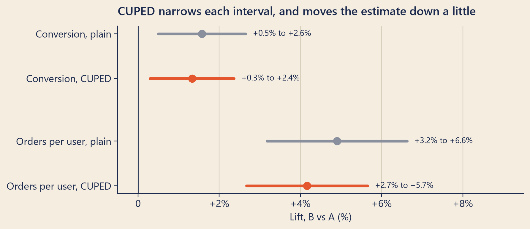
For conversion, the correlation between app visits before the test and conversion during it was 0.26. (A correlation of 0 means no link and 1 means a perfect straight-line link.) Variance is the square of the standard deviation (Chapter 16): a measure of how much the users’ outcomes spread out. CUPED removes about the square of the correlation from it: 0.26 × 0.26 ≈ 7% of the variance. The interval became 3.7% narrower.
The estimate also moved, from +1.57% to +1.33%, and the p-value rose from 0.004 to 0.011. This is group B’s head start at work. B had slightly more active users, and active users order more. CUPED took out the part of B’s lead that its users’ past already explained. The rest is still a clear win: the interval stays above zero.
“Wait,” Priya said. “The faster method made the p-value bigger?”
“It made the measurement more careful,” Mia said. “Plain, the test gave the new checkout a little credit for a lucky draw of users. CUPED took that credit back.”
This is the most important thing to know about CUPED. It is not a machine for smaller p-values. Most of the time it does shrink them, because it removes noise. But when chance gave one group a head start, it also corrects the estimate. CUPED’s number is not the truth either, but it depends less on the luck of who landed in which group.
For orders per user, the past predicts the future better. The correlation was 0.49, the variance cut 24%, and the interval 13% narrower. A yes-or-no outcome over two weeks is harder to predict: many light users still order once.
Show the code
items = [("Conversion, plain", conv["plain"], bk.MUTED), ("Conversion, CUPED", conv["cuped"], bk.TOMATO), ("Orders per user, plain", orders["plain"], bk.MUTED), ("Orders per user, CUPED", orders["cuped"], bk.TOMATO)]fig, ax = bk.figure(8, 3.4)for k, (label, (mid, lo, hi, _), color) inenumerate(items): y = k + (0.4if k >=2else0) ax.plot([100* lo, 100* hi], [y, y], color=color, lw=3, solid_capstyle="round") ax.plot(100* mid, y, "o", color=color, ms=8) ax.annotate(f"{pct(lo)} to {pct(hi)}", (100* hi, y), xytext=(8, 0), textcoords="offset points", va="center", fontsize=9)ax.axvline(0, color=bk.INK, lw=0.9)ax.set_yticks([0, 1, 2.4, 3.4], [i[0] for i in items])ax.invert_yaxis()ax.grid(axis="y", visible=False)ax.grid(axis="x")ax.set_xlim(-0.5, 9.5)ax.xaxis.set_major_formatter(mticker.FuncFormatter(lambda v, _: f"{v:+.0f}%"if v else"0"))ax.set_xlabel("Lift, B vs A (%)")ax.set_title("CUPED narrows each interval, and moves the estimate down a little")plt.show()
Figure 1: Relative lift with 95% intervals for checkout_v2, plain and with CUPED (covariate: app visits in the two weeks before the test).
How many days is that worth?
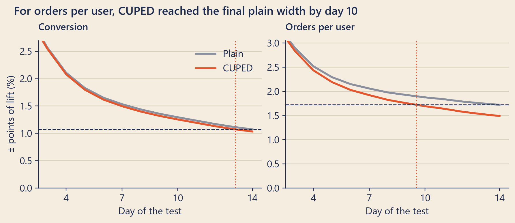
A narrower interval at the same end date is one way to spend the gain. The other is to reach the same width sooner. To measure that, Mia replayed the test day by day, as she had done for the price test (Chapter 21): on each day, every user who had joined so far, with what they had done so far.
Show the code
bk.setup()fig, axes = plt.subplots(1, 2, figsize=(8, 3.4), layout="constrained", sharey=False)for ax, (title, path, catch) inzip(axes, [("Conversion", conv_path, conv_catch), ("Orders per user", ord_path, ord_catch)]): days = path.index.to_numpy() ax.plot(days, 100* Z95 * path.se, color=bk.MUTED, lw=2.2, label="Plain") ax.plot(days, 100* Z95 * path.se_cuped, color=bk.TOMATO, lw=2.2, label="CUPED") target =100* Z95 * path.se.iloc[-1] ax.axhline(target, color=bk.INK, ls="--", lw=1) ax.axvline(catch, color=bk.TOMATO, ls=":", lw=1.2) ax.set_title(title, fontsize=11) ax.set_xlabel("Day of the test") ax.set_xticks([1, 4, 7, 10, 14]) ax.set_ylim(0, 100* Z95 * path.se.iloc[2] *1.05) ax.set_xlim(2.5, 14.5)axes[0].set_ylabel("± points of lift (%)")axes[0].legend(loc="upper right")fig.suptitle(f"For orders per user, CUPED reached the final plain width by day {ord_catch_day}", x=0.02, ha="left", fontweight="semibold", fontsize=13)plt.show()
Figure 2: Half-width of the 95% interval for the relative lift, day by day, plain and with CUPED. The dashed line is the plain width on the last day.
For conversion, CUPED reached the plain test’s final width less than a day before the end: a saving of about 0.9 days out of 14. For orders per user, it got there on day 10, about 4 days sooner.
Why so little for conversion? One more day of the test narrowed the plain interval by about 4%. CUPED makes it 3.7% narrower. So, for conversion, CUPED is worth a little less than one day. Steep’s tests also run in whole weeks, to cover each weekday equally (Chapter 19). So for conversion, Mia would keep two weeks and use CUPED for a sharper answer. For a metric like orders per user, the gain can be planned in: a smaller MDE, or fewer users, from the start. It would not have rescued Priya’s wish from Chapter 19, a two-week test that sees a 1% lift in conversion. Halving the MDE takes about four times the users (Chapter 19), and CUPED on conversion is worth only 7% more.
When CUPED fails
No history, no help. CUPED needs a past. In checkout_v2, 10,258 users (15%) had made no app visit in the two weeks before the test. Of these, 1,235 had not even signed up yet: they joined Steep during the test. For all of them, the covariate is zero. CUPED shifts them all by the same amount, so inside this group it removes none of the noise. A test of a sign-up screen, where every user is new, would get no help at all. Covariates that exist from the first moment, such as city and platform, can help a little there.
A covariate measured after the coin. If you adjust for something the treatment can change, you remove part of the real effect, or add a false one. App visits during the test are not allowed, even though they would correlate even better. Use only data from before each user’s exposure.
A weak link. The gain is about the square of the correlation. A correlation of 0.1 cuts the variance by only 1%. Look for the covariate that predicts the metric best. Often it is the same metric, measured before the test.
NoteUnder the hood
Let \(Y\) be the outcome and \(X\) the covariate, measured before exposure. CUPED uses
where \(\rho\) is the correlation between \(Y\) and \(X\); \(\theta\) is the value that makes this variance smallest. For conversion here, \(\rho^2\) = 0.067 and the measured cut was 0.067.
Because \(X\) was fixed before the coin was flipped, \(E[\bar X_B - \bar X_A] = 0\), so the adjustment adds no bias on average. In one test, it subtracts the part of the gap that the covariate explains: here, B’s head start.
A test with variance \((1 - \rho^2)\sigma^2\) is as precise as a plain test with \(1 / (1 - \rho^2)\) times as many users. With one covariate, CUPED gives almost the same answer as a regression of \(Y\) on the group and \(X\); with several covariates, use that regression.
Try it: CUPED, before and after
The playground runs on the real checkout_v2 user file, in your browser. Choose the metric, the covariate, and which users to include. Try “Users with no history”: the covariate is zero for all of them, and CUPED does nothing.
Show the code
viewof c22Cuped = Inputs.form({metric: Inputs.select(newMap([ ["Conversion (primary)","case when converted then 1.0 else 0.0 end"], ["Orders per user","orders::double"], ["Revenue per user","net_revenue::double"] ]), {label:"Metric"}),covariate: Inputs.select(newMap([ ["App visits before the test","pre_sessions::double"], ["Orders before the test","pre_orders::double"], ["Revenue before the test","pre_net_revenue::double"], ["Drinks before the test","pre_items::double"], ["None (plain test)","0.0"] ]), {label:"Covariate"}),who: Inputs.radio(newMap([ ["All users","true"], ["Users with history","pre_sessions > 0"], ["Users with no history","pre_sessions = 0"] ]), {value:"true",label:"Users"})})
Show the code
c22CupedView = {const r = c22CupedStats;const f = (x, d =2) => (x >=0?"+":"−") +Math.abs(100* x).toFixed(d) +"%";const p = (v) => v <0.001?"p < 0.001":`p = ${v.toFixed(3)}`;const rows = [ {label:"Plain",lift: r.plain.lift,lo: r.plain.lo,hi: r.plain.hi}, {label:"CUPED",lift: r.cuped.lift,lo: r.cuped.lo,hi: r.cuped.hi} ];const chart = Plot.plot({width:Math.min(width,640),height:140,marginLeft:60,style: {background:"transparent",fontSize:"12px"},x: {label:"Relative lift, B vs A (%) →",tickFormat: (d) => d >0?`+${d}`: d <0?`−${-d}`:"0"},y: {label:null,domain: ["Plain","CUPED"]},marks: [ Plot.ruleX([0], {stroke:"#1d2b4f"}), Plot.link(rows, {x1: (d) =>100* d.lo,x2: (d) =>100* d.hi,y1:"label",y2:"label",stroke: (d) => d.label==="CUPED"?"#e4572e":"#8a8f9e",strokeWidth:4}), Plot.dot(rows, {x: (d) =>100* d.lift,y:"label",r:6,fill: (d) => d.label==="CUPED"?"#e4572e":"#8a8f9e"}) ] });const note = r.noCovariate?html`<p>The covariate is the same for every user here, so CUPED has nothing to work with: both rows are the same.</p>`:html`<p>Correlation with the metric: <strong>${r.rho.toFixed(2)}</strong>. Variance cut: <strong>${(100* r.cut).toFixed(1)}%</strong>, worth about <strong>${(100* (1/ (1- r.cut) -1)).toFixed(0)}%</strong> more users. Interval <strong>${(100* (1- (r.cuped.hi- r.cuped.lo) / (r.plain.hi- r.plain.lo))).toFixed(1)}%</strong> narrower.</p>`;returnhtml`<p><strong>${r.n.toLocaleString("en-US")}</strong> users. Plain: <strong>${f(r.plain.lift)}</strong> (${f(r.plain.lo)} to ${f(r.plain.hi)}), ${p(r.plain.p)}.<br> CUPED: <strong>${f(r.cuped.lift)}</strong> (${f(r.cuped.lo)} to ${f(r.cuped.hi)}), ${p(r.cuped.p)}.</p>${note}${chart}`;}
Show the code
c22Db = DuckDBClient.of({users:FileAttachment("../data/out/web/ads_experiment_user_checkout_v2.parquet")})c22CupedRows = c22Db.query(` select variant, count(*)::double as n, sum(y)::double as sy, sum(y * y)::double as syy, sum(x)::double as sx, sum(x * x)::double as sxx, sum(x * y)::double as sxy from (select variant, (${c22Cuped.metric})::double as y, (${c22Cuped.covariate})::double as x from users where ${c22Cuped.who}) t group by variant order by variant`)c22CupedStats = {const [A, B] = c22CupedRows.map((r) =>Object.fromEntries(Object.entries(r).map(([k, v]) => [k,typeof v ==="bigint"?Number(v) : v])));const N = A.n+ B.n;const yBar = (A.sy+ B.sy) / N, xBar = (A.sx+ B.sx) / N;const varX = (A.sxx+ B.sxx- N * xBar **2) / (N -1);const varY = (A.syy+ B.syy- N * yBar **2) / (N -1);const cov = (A.sxy+ B.sxy- N * xBar * yBar) / (N -1);const noCovariate =!(varX >1e-12);const theta = noCovariate ?0: cov / varX;// One group: its mean and variance after the adjustment y - theta * (x - xBar).const arm = (g, th) => {const my = g.sy/ g.n, mx = g.sx/ g.n;const vy = (g.syy- g.n* my **2) / (g.n-1);const vx = (g.sxx- g.n* mx **2) / (g.n-1);const cxy = (g.sxy- g.n* mx * my) / (g.n-1);return {n: g.n,mean: my - th * (mx - xBar),v: vy -2* th * cxy + th * th * vx}; };const result = (th) => {const a =arm(A, th), b =arm(B, th);const lift = b.mean/ a.mean-1;const se =Math.sqrt(b.v/ b.n/ a.mean**2+ b.mean**2* a.v/ a.n/ a.mean**4);const z = (b.mean- a.mean) /Math.sqrt(a.v/ a.n+ b.v/ b.n);return {lift,lo: lift -1.959964* se,hi: lift +1.959964* se,p:c22P(z)}; };return {n: N, noCovariate, theta,rho: noCovariate ?0: cov /Math.sqrt(varX * varY),cut: noCovariate ?0:1- (varY -2* theta * cov + theta * theta * varX) / varY,plain:result(0),cuped:result(theta) };}
Part 2 · Look often, honestly: sequential testing
A budget for false alarms
Chapter 21 showed why peeking fails. With a line at p = 0.05 and a look every day for 14 days, about 22% of A/A tests raise a false alarm at least once, not 5%. Each look is another chance for noise to cross the line.
A sequential test is a test designed for many looks. It moves the line so that the chance of any false alarm, over all the looks together, stays at alpha. The usual way to think about it is alpha spending. Alpha, the 5%, is a budget. Every look spends some of it. When the budget is gone, the test is over.
A z-score here is the difference between B and A divided by its standard error: how many standard errors apart the groups are. The usual one-look test calls a result significant when it is beyond ±1.96. There are two classic ways to spend the budget.
A Pocock-type plan uses the same strict line at every look. For 14 equal daily looks, that line is z = 2.62 (p < 0.009) every day.
An O’Brien–Fleming-type plan spends almost nothing early and saves most of the budget for the end. For 14 equal looks, the line starts at z = 7.9 on day 1, is 2.98 on day 7, and ends at 2.10 (p < 0.035) on the last day. The final line is only a little stricter than the usual 1.96.
In a real test, each look may spend alpha according to how much the test has learned so far, not how many days have passed. By day 3 of checkout_v2, 48% of the users had joined, but their two weeks had barely begun: conversion so far was 43%, not 66%. The estimate was still far less precise than it would be at the end. Under the hood shows how the lines are set.
What would have stopped checkout_v2?
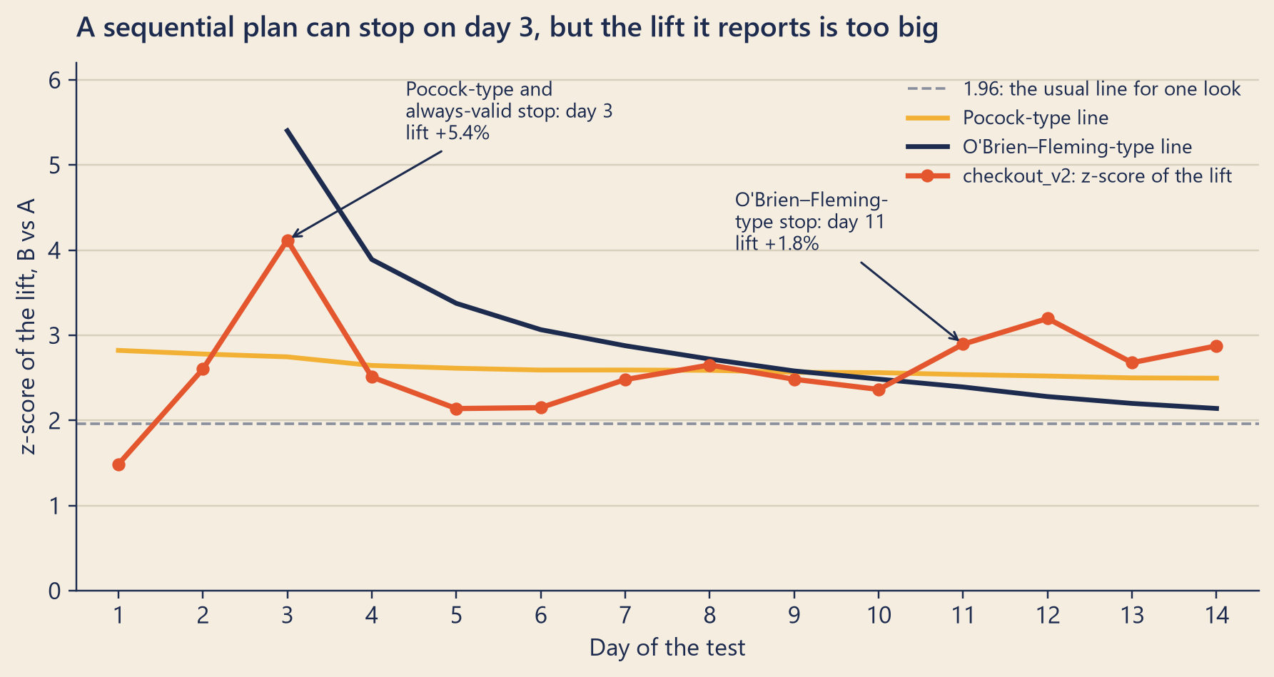
Mia replayed checkout_v2 day by day. For each day she divided the lift in conversion by its standard error, the z-score of the lift, and drew it against each kind of line.
Show the code
fig, ax = bk.figure(8, 4.2)days = conv_path.index.to_numpy()ax.axhline(Z95, color=bk.MUTED, ls="--", lw=1.2, label="1.96: the usual line for one look")ax.plot(days, pocock_daily, color=bk.MUSTARD, lw=2.2, label="Pocock-type line")show = np.isfinite(obf_daily)ax.plot(days[show], obf_daily[show], color=bk.INK, lw=2.2, label="O'Brien–Fleming-type line")ax.plot(days, z, color=bk.TOMATO, lw=2.4, marker="o", ms=5, label="checkout_v2: z-score of the lift")for key, label, spot in [("pocock", "Pocock-type and\nalways-valid stop", (4.4, 5.3)), ("obf", "O'Brien–Fleming-\ntype stop", (8.3, 4.0))]: d = stops[key] ax.annotate(f"{label}: day {d}\nlift {pct(stop_lift[key])}", xy=(d, z.loc[d]), xytext=spot, arrowprops=dict(arrowstyle="->", color=bk.INK), fontsize=9)ax.legend(loc="upper right", fontsize=9)ax.set_ylim(0, 6.2)ax.set_xlim(0.5, 14.5)ax.set_xticks(range(1, 15))ax.set_xlabel("Day of the test")ax.set_ylabel("z-score of the lift, B vs A")ax.set_title("A sequential plan can stop on day 3, but the lift it reports is too big")plt.show()
Figure 3: The z-score of the relative lift in conversion for checkout_v2 (the lift divided by its standard error), day by day, against the lines of two sequential plans (alpha = 0.05, each line set by how precise the estimate was that day). The usual one-look line, 1.96, is dashed.
Plan
Stops on
Lift in conversion it reports
Look once, after day 14 (the plan in Chapter 20)
day 14
+1.6%
Peek every day at the usual 1.96 line (not valid)
day 2
+4.1%
Pocock-type, a look every day
day 3
+5.4%
Always-valid p-value, checked every day
day 3
+5.4%
O’Brien–Fleming-type, a look every day
day 11
+1.8%
O’Brien–Fleming-type, a look at the end of each week
day 14
+1.6%
Every valid plan in the table finds the effect. The new checkout does help, and none of them is fooled. But look at the sizes. The z-score jumped on day 3, when the lift in conversion so far was +5.4%. A plan that stops at that moment reports +5.4%: 3.4 times the two-week +1.6%. That factor has two parts. The gap in points was 2.30 on day 3 against 1.04 at the end: 2.2 times as big. And the base was smaller: 43% of group A had ordered by day 3, against 66% at the end, which makes the same points 1.5 times bigger as a share. Together: 2.21 × 1.55 ≈ 3.42. Part of the gap in points is luck: a test usually stops early because it hit a lucky high point. Either way, a decision made on day 3 would have carried a number that does not hold. It is Chapter 19’s winner’s curse again: a result that crosses a line early is usually one that luck pushed up.
The O’Brien–Fleming-type plan with daily looks stopped on day 11, a Thursday, with a lift close to the final one. But stopping in the middle of a week means some weekdays count twice and some once. With one look at the end of each week, it ran the full two weeks, as Mia’s plan did.
Always-valid p-values
There is a second family of methods. An always-valid p-value may be checked after every new user, as often as you like. If there is no real effect, the chance that it ever drops below 5% is at most 5%. One version is the mSPRT (Johari and colleagues, 2017). The price is power: to be safe at every moment, its line must be stricter than 1.96. For checkout_v2 it crossed on day 3, with the same inflated lift. On day 14 alone, its line was z = 3.05, above the test’s z of 2.90. So without the day-3 spike it would never have called a win. Always-valid p-values suit questions you must watch all the time, such as guardrails; plans with a few fixed looks suit the main decision.
Priya’s plan
“So for my offer,” Priya said, “what do I actually do?”
Mia wrote it on the second page of her notebook.
Size the test first, as in Chapter 19. Say it needs four weeks.
Look once a week, at the end of each week, so every look covers whole weeks.
Use O’Brien–Fleming-type lines. For four weekly looks, stop early for a win only if p < 0.00005 after week 1, p < 0.0042 after week 2, or p < 0.019 after week 3. At the end of week 4, the line is p < 0.043.
If it stops early, say the size is probably too big, and keep a holdout to measure it again.
Watch the guardrails every day with an always-valid p-value, and stop at once for clear harm.
Mia checked the cost with a simulation. Suppose the true effect is exactly the MDE. A plain test with one look after four weeks finds it 80% of the time. Priya’s plan finds it 79% of the time, and on average it ends after 3.3 weeks instead of four. If there is no effect, it runs the full four weeks almost every time. B wins falsely only about 2.6% of the time. That is about the same as a plain two-sided test at 5%, where half of the false alarms favour B.
“That’s the honest version of looking early,” Priya said.
“It is,” Mia said. “You may look. But you have to decide in advance what you will do with each look.”
NoteUnder the hood
Alpha spending. Let \(t \in (0, 1]\) be the information fraction: the share of the final information seen so far, that is, how precise the estimate is so far compared with the end. For checkout_v2 it was about 18% on day 3. This chapter uses the standard error of the relative lift, \(t_k = \mathrm{SE}_{\text{final}}^2 / \mathrm{SE}_k^2\), and tests the z-score of the lift, \(\widehat{\text{lift}}_k / \mathrm{SE}_k\). (The difference in points is a poor guide here, because it grows as conversion grows.) The formula assumes that each user’s outcome is finished when it is counted. In this replay outcomes keep growing, so it is approximate. A check that uses the real correlation between the looks gives the same stopping days, and shows that these lines’ real false-alarm rate is about 5.8% rather than 5%. A spending function\(\alpha(t)\) says how much of alpha may be used up by time \(t\). The two classic choices are
At each look \(k\), the boundary \(c_k\) is chosen so that, with no real effect, \(P(\text{first crossing at look } k) = \alpha(t_k) - \alpha(t_{k-1})\). The z-scores at different looks are related: \(Z_k = W(t_k)/\sqrt{t_k}\) for a Brownian motion \(W\), so the boundaries come from that joint distribution. This chapter finds them by simulating 400,000 paths. The table for the playground uses equal looks, \(t_k = k/K\), and the constant-line (Pocock) and \(c\sqrt{K/k}\) (O’Brien–Fleming) shapes of Chapter 21.
mSPRT. Let \(\hat\Delta_n\) be the difference in means after \(n\) users, with variance \(s_n^2\). Mixing over true effects \(\Delta \sim N(0, \tau^2)\) gives the likelihood ratio
With no effect, \(\Lambda_n\) is a martingale with mean 1, so by Ville’s inequality \(P(\sup_n \Lambda_n \ge 1/\alpha) \le \alpha\). The always-valid p-value is \(p_n = \min\big(1, \min_{m \le n} 1/\Lambda_m\big)\). Mia set \(\tau\) to the plan’s MDE as a difference in conversion: 0.0132 as a share, that is 1.32 points. The mSPRT here works on that difference, \(\hat\Delta_n\), also as a share.
One caution. In this replay each user’s outcome keeps growing as the test runs (“converted by day d”), so the data are not a simple stream of finished observations. The mSPRT guarantee, like the spending functions, holds exactly for finished observations and approximately here.
Try it: a boundary for many looks
Each line below is one simulated test. Choose how many looks, which line to use, and whether there is a real effect. “The MDE” is an effect that a single look at the end would find 80% of the time.
c22SeqPlot = {const {looks} = c22Seq;const rows = [], ends = []; c22Sim.paths.slice(0,30).forEach((p, test) => {const stop = p.stop?? looks;for (let k =1; k <= stop; k++) rows.push({test,look: k,z: p.z[k -1],status: p.stop? (p.win?"stopped: B better":"stopped: A better") :"ran to the end"});if (p.stop) ends.push(rows[rows.length-1]); });const line =Array.from({length: looks}, (_, i) => ({look: i +1,z: c22Sim.line[i]}));return Plot.plot({width:Math.min(width,640),height:320,marginLeft:44,style: {background:"transparent",fontSize:"12px"},x: {label:"Look →",domain: [1,Math.max(2, looks)]},y: {label:"↑ z-score, B vs A",domain: [-5,7],tickFormat: (d) => d <0?`−${-d}`:`${d}`},color: {domain: ["ran to the end","stopped: B better","stopped: A better"],range: ["#8a8f9e","#e4572e","#2a9d8f"],legend:true},marks: [ Plot.ruleY([0], {stroke:"#d9cfbd"}), Plot.line(line, {x:"look",y:"z",stroke:"#1d2b4f",strokeWidth:2,clip:true}), Plot.line(line, {x:"look",y: (d) =>-d.z,stroke:"#1d2b4f",strokeWidth:2,clip:true}), Plot.line(rows, {x:"look",y:"z",z:"test",stroke:"status",strokeOpacity:0.75,strokeWidth:1.2,clip:true}), Plot.dot(ends, {x:"look",y:"z",fill:"status",r:3.5,clip:true}) ] });}
Show the code
c22SeqReadout = {const s = c22Sim, {effect, alpha} = c22Seq;const pc = (x) =>`${(100* x).toFixed(1)}%`;if (effect ===0) {returnhtml`<p>Showing 30 of ${s.n.toLocaleString("en-US")} A/A tests: every alarm is false.</p> <ul><li>This plan: <strong>${pc(s.stopRate)}</strong> false alarms.</li> <li>One look at the end: <strong>${pc(s.fixedRate)}</strong>.</li></ul> <p>The promise was ${pc(Number(alpha))}.</p>`; }returnhtml`<p>Showing 30 of ${s.n.toLocaleString("en-US")} tests with a real effect.</p> <ul><li>This plan found it in <strong>${pc(s.winRate)}</strong> of tests. On average a test ran <strong>${s.meanStop.toFixed(1)}</strong> of ${c22Seq.looks} looks.</li> <li>One look at the end found it: <strong>${pc(s.fixedWin)}</strong>.</li> <li>When this plan found it, the size it reported was on average <strong>${s.exaggeration.toFixed(2)} ×</strong> the true effect.</li></ul>`;}
functionc22Mulberry(seed) {let s = seed >>>0;return () => { s = (s +0x6D2B79F5) >>>0;let t = s; t =Math.imul(t ^ (t >>>15), t |1); t ^= t +Math.imul(t ^ (t >>>7), t |61);return ((t ^ (t >>>14)) >>>0) /4294967296; };}// Standard normal numbers from uniform ones (Box-Muller).functionc22Gaussian(random) {return () => {let u =0;while (u ===0) u =random();returnMath.sqrt(-2*Math.log(u)) *Math.cos(2*Math.PI*random()); };}// Two-sided p-value of a z-score: erfc(|z| / sqrt 2), Abramowitz and Stegun 7.1.26.functionc22P(z) {const x =Math.abs(z) /Math.SQRT2;const t =1/ (1+0.3275911* x);const poly = t * (0.254829592+ t * (-0.284496736+ t * (1.421413741+ t * (-1.453152027+ t *1.061405429))));returnMath.min(1, poly *Math.exp(-x * x));}
Try “The MDE” with the O’Brien–Fleming-type line, then with Pocock-type. Pocock-type stops sooner but finds the effect less often. Then look at the last line of the readout: the earlier a plan tends to stop, the more it overstates the size.
Part 3 · Bayesian A/B testing in plain terms
So far every test in this book has asked one question: if there were no difference, how surprising would this data be? That is the p-value. Priya’s next question was the one many managers really want answered.
“Can’t you tell me the chance that B is better?”
You can, with Bayesian statistics. It starts from a prior: what you believe about the effect before the test, written as a range of possible values with weights. The data then update the prior into a posterior: what you believe after seeing the data. From the posterior you can read off direct answers.
For checkout_v2, with a flat prior (every conversion rate equally likely before the test), the posterior says:
The chance that B is better: 99.8%. With a flat prior and this much data, this is close to 1 minus the one-sided p-value: 1 − 0.002.
A 95% credible interval for the relative lift, the range that holds the true lift with 95% probability under this prior: +0.5% to +2.7%. With this much data and a flat prior, it is almost the same as Chapter 20’s confidence interval.
The expected loss of choosing B: the conversion you would give up, averaged over all the possibilities, counting zero whenever B is better. Here it is about 0.0002 points: almost nothing.
The prior matters when data are thin, and it can be honest about experience. Most product changes move a metric by a little, if at all. A sceptical prior says so: before the test, Mia might say the lift is probably within about ±2%, a normal curve centred on zero with a spread of 1%. With that prior, the posterior pulls the estimate toward zero: +1.2% instead of +1.6%. The chance that B is better is still 99.4%.
It does not make peeking free
A common claim is that Bayesian tests let you look as often as you like. They do not, if “looking” means stopping when the number looks good. Take the rule “ship B as soon as the chance that B is better passes 95%”. A usual two-sided 5% test gives B a false win only 2.5% of the time. “P(B better) > 95%” gives B 5%, even with one look. Mia then checked it every day on the 200,000 A/A tests of Chapter 21, where B is never better: B “won” 19% of them.
The posterior on any one day is a correct summary of that day’s data. But a rule that keeps checking until the answer is “yes” will find “yes” more often by chance. The fix is the same as before: decide the looks and the rule in advance, and check what the rule does on A/A tests.
Common traps
Adjusting for something the treatment can change. A covariate must be measured before each user’s exposure. Otherwise CUPED can remove the very effect you want to measure.
Treating CUPED as a p-value booster. It removes noise and corrects chance imbalance. Sometimes the estimate goes down, as it did here. Use it when the plan says so. CUPED was not in the plan for checkout_v2, so the decision stands on the planned analysis, and CUPED is a second look.
Choosing the analysis after the results. Decide in the plan whether you will use CUPED, with which covariate, and how many looks. Picking the best-looking of several analyses is Lie 2 of Chapter 21 in a new form.
Trusting the size at an early stop. Sequential tests protect the yes-or-no answer, not the size. An early stop usually overstates the effect.
Stopping in the middle of a week. Daily looks can stop on a Thursday. Weekly looks keep every weekday equally represented.
“Bayesian, so I can peek.” A posterior is not a licence to stop whenever it looks good. Check your stopping rule on A/A tests.
TipAudit Instinct · Last year’s file and the risk assessment
Auditors do not start each year from nothing. They read last year’s working papers and their knowledge of the client to assess risk: where errors are likely, and how large. Where the risk is low and well understood, they can test less. Where it is high, they test more, or test differently. Last year’s knowledge does not change this year’s facts. It tells them where to look and how much evidence they need.
CUPED is the same habit. Each user’s behaviour before the test is last year’s file. It does not change what happened during the test. It tells you which part of each user’s result was already expected, so that the evidence you collect goes further. And as in audit, prior knowledge must come from before the period under test: a covariate from after the coin is like letting this year’s findings rewrite last year’s file.
NoteInterview Corner
1. What is CUPED and when does it help?
NoteA model answer
CUPED adjusts each user’s outcome by a covariate measured before the test, usually the same metric in a pre-period: \(Y - \theta(X - \bar X)\), with \(\theta = \operatorname{Cov}(Y, X)/\operatorname{Var}(X)\). It cuts the variance by about \(\rho^2\), the squared correlation, without bias, because the covariate cannot be affected by the treatment. It helps most for metrics that the past predicts well, such as orders or revenue per user, and little for weakly predictable ones or for new users with no history. It can also move the estimate, when chance gave one group a head start. In checkout_v2 it cut the variance of orders per user by 24%, but of conversion by only 6.7%.
2. How can you stop a test early safely?
NoteA model answer
Use a sequential design chosen before the test: a group-sequential plan with an alpha-spending function, usually O’Brien–Fleming-type, which keeps the overall false-positive rate at alpha and loses little power; or an always-valid method such as mSPRT for continuous monitoring. Look at whole-week boundaries if the metric has a weekly cycle. Expect the effect size at an early stop to be overstated, and confirm it with a holdout. Guardrails can be monitored continuously, and a test stopped at once for clear harm.
3. Frequentist vs Bayesian A/B testing?
NoteA model answer
A frequentist test asks how surprising the data would be if there were no effect, and controls the error rate of a decision rule. A Bayesian analysis combines a prior with the data and reports direct statements, such as the probability that B is better and the expected loss of choosing B. With a lot of data and a weak prior, the two usually agree. A sceptical prior can protect against overestimating small effects. Neither makes repeated peeking free: a stopping rule must be checked for its false-positive rate either way.
Reported change: −12.0% orders, the week of 7 September compared with the week before (CEO dashboard).
Explained so far: 12.0 of the 12 points (closed in Chapter 21): the tracking bug 7.0 (Chapter 15), the rainy week before 3.4 and normal growth −0.3 (Chapter 16), and the price rise for everyone on 7 September 1.9 (Chapter 21).
Suspects: the 5% price rise for everyone on 7 September: proved (Chapter 21).
Ruled out: the matcha menu (Chapter 4); every stop on the data’s journey after the app (Chapters 8–14); Priya’s day-3 “win” (peeking, Chapter 21).
Open questions: Did Riverside’s delivery fee since 5 October cost orders? (Chapter 23.) How to tell the board of directors (Chapter 24).
Recap
CUPED uses each user’s behaviour before the test to remove predictable noise. It needs a pre-exposure covariate and a history; it helps most when the past predicts the metric well, and it can correct a chance head start.
To look early, plan the looks and the lines in advance: O’Brien–Fleming-type spending for decisions, always-valid p-values for continuous watching. An early stop protects the answer, not the size.
A Bayesian analysis gives direct answers, such as the chance that B is better, but a rule that checks it until it says yes still raises false alarms.
English
中文
CUPED
CUPED(利用实验前数据的方差缩减)
variance reduction
方差缩减
covariate
协变量
pre-period
实验前时期
correlation
相关系数
sequential testing
序贯检验
alpha spending
α 消耗
information fraction
信息比例
O’Brien–Fleming / Pocock boundary
O’Brien–Fleming / Pocock 边界
always-valid p-value
始终有效的 p 值
Bayesian
贝叶斯
prior
先验
posterior
后验
credible interval
可信区间
expected loss
期望损失
Further reading
Deng, A., Xu, Y., Kohavi, R., & Walker, T. (2013). Improving the Sensitivity of Online Controlled Experiments by Utilizing Pre-Experiment Data. Proceedings of the Sixth ACM International Conference on Web Search and Data Mining (WSDM), 123–132. DOI. The CUPED paper.
Johari, R., Koomen, P., Pekelis, L., & Walsh, D. (2017). Peeking at A/B Tests: Why It Matters, and What to Do About It. Proceedings of the 23rd ACM SIGKDD International Conference on Knowledge Discovery and Data Mining, 1517–1525. DOI. Always-valid p-values and the mSPRT.
Kohavi, R., Tang, D., & Xu, Y. (2020). Trustworthy Online Controlled Experiments: A Practical Guide to A/B Testing. Cambridge University Press. DOI. Variance reduction, sequential tests and their trade-offs in practice.