On Monday 12 October, the case board had one line left. In points of the 12% drop: about 7.0 were the tracking bug (Chapter 15), about 3.4 the rainy week before, and normal weekly growth pushed the other way by 0.3 (Chapter 16). That left about 1.9 points open.
Mia’s suspect was the 5% price rise for everyone on 7 September (Chapter 18). But the weekly numbers could not tell those 1.9 points from noise (two-sided p = 0.191; range about −0.7 to 4.5 points). As Chapter 19 showed, weekly totals had only about 33% power, the chance to see a real 2% drop in orders. Priya’s price test, read after all 14 days, had about 64%: the strongest evidence Steep had.
So Mia went to find Priya. She was at the long table by the window, eating noodles in front of her laptop.
“Can I ask you about price_up_5?” Mia said.
“My favourite test.” Priya turned the laptop around. “I even kept the message.”
The test started on 10 August: half of the users, chosen at random, saw prices 5% higher. The message was from 12 August, the third day:
Priya: Day 3 of price_up_5. Revenue per user is up +4.8% with the new prices, p = 0.002. Significant! Shipping it.
“Everybody was happy,” Priya said. “The launch had to wait for the engineers’ next work cycle, so the test kept running for its planned 14 days. Then, on 7 September, the new prices went to everyone.”
“Did anyone look at the test again after day 3?”
Priya put down her chopsticks. “Why would we? It had already won.”
Mia wrote in her notebook: Day 3: one look, with about 29% power for a 2% change in orders. Days 4 to 14: never read. Her own checkout_v2 had been read once, at its planned end (Chapter 20).
Priya is not careless. She is smart and honest, and she did what most people do: she looked early, saw a small p-value, and believed it. Mia opened the test data and ran it again, this time with all fourteen days.
Reminders for skimmers. A/B tests and their parts are in Chapter 20. A p-value is the chance of a difference at least this large if nothing had changed, not the chance that your idea is right (Chapter 18). A false positive is noise that looks real; alpha, usually 5%, is how often you accept one (Chapter 18). Here, users are app users: people who opened the app while the test ran.
ImportantThe big idea
An A/B test tells the truth only if you follow your plan: check that the split was fair, then ask your one planned question once, at the planned end, or use a method built for many looks.
Lie 1 · Peeking
What it looked like at Steep
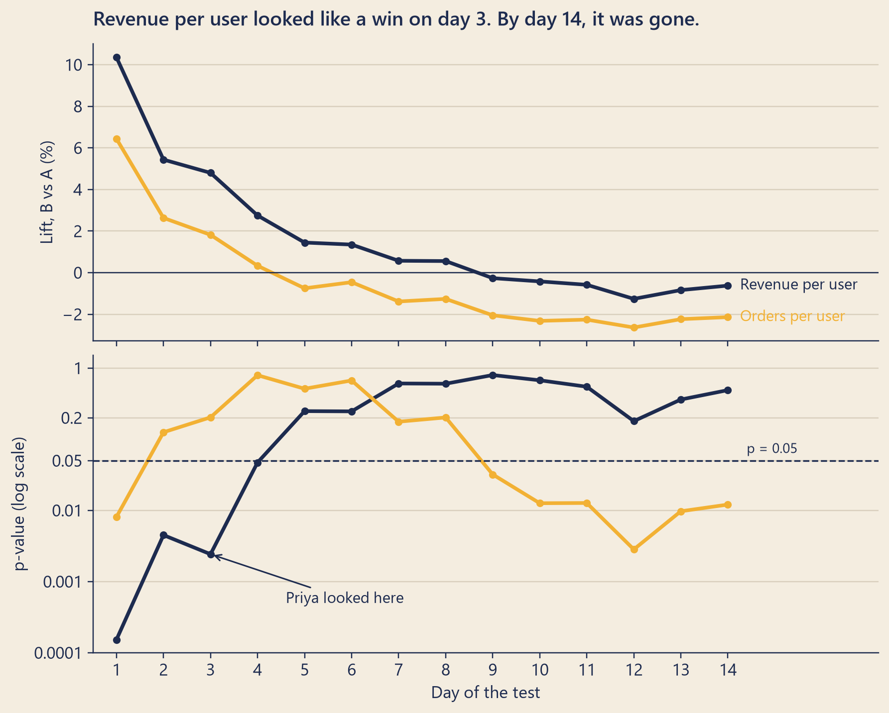
Mia replayed the test the way Priya saw it: each day, every user who had joined so far, with everything they had spent so far. The top chart shows the lift, how much higher B is than A as a percentage of A. The bottom chart has a log scale: each step up is ten times bigger.
Show the code
bk.setup()fig, (top, bottom) = plt.subplots(2, 1, figsize=(8, 6.4), sharex=True, layout="constrained")for path, label, color in [(rev_path, "Revenue per user", bk.INK), (ord_path, "Orders per user", bk.MUSTARD)]: top.plot(path.day, 100* path.lift, color=color, lw=2.4, marker="o", ms=4) bottom.plot(path.day, path.p, color=color, lw=2.4, marker="o", ms=4) top.annotate(label, (path.day.iloc[-1], 100* path.lift.iloc[-1]), xytext=(8, 0), textcoords="offset points", color=color, va="center", fontsize=10)top.axhline(0, color=bk.INK, lw=0.8)top.set_ylabel("Lift, B vs A (%)")top.set_title(f"Revenue per user looked like a win on day 3. By day {n_days}, it was gone.")bottom.axhline(0.05, color=bk.INK, ls="--", lw=1.1)bottom.text(n_days +0.4, 0.058, "p = 0.05", va="bottom", fontsize=9)bottom.annotate("Priya looked here", xy=(3, day3.p), xytext=(4.6, 0.0005), arrowprops=dict(arrowstyle="->", color=bk.INK), fontsize=10)bottom.set_yscale("log")bottom.set_ylim(1e-4, 1.5)bottom.set_yticks([0.0001, 0.001, 0.01, 0.05, 0.2, 1])bottom.yaxis.set_major_formatter(mticker.FuncFormatter(lambda v, _: f"{v:g}"))bottom.yaxis.set_minor_locator(mticker.NullLocator())bottom.set_ylabel("p-value (log scale)")bottom.set_xlabel("Day of the test")bottom.set_xticks(range(1, n_days +1))bottom.set_xlim(0.5, n_days +3.2)plt.show()
Figure 1: Mia’s replay of the price test. Each point uses every user who had joined by the end of that day, and everything they had done so far.
On day 3, the day Priya looked, the lead was +4.8% and p was 0.002. The p-value stayed below 0.05 for the first 4 days. After day 4, the lowest the p-value reached was 0.18. On day 14, the lift in revenue per user was −0.6%, with p = 0.489.
Orders per user even went the wrong way on day 1: up +6.4%, p = 0.008. By the end, it was clearly down: −2.1%, p = 0.012.
The early days rest on little data: on day 1, only 13,351 users had joined, with one day each. By day 14, there were 64,568.
Try it: look on any day
Pick a day and a metric to see what someone who looked then saw.
Show the code
viewof lookDay = Inputs.range([1,14], {value:3,step:1,label:"Look on day"})viewof lookMetric = Inputs.radio(newMap([["Revenue per user","net_revenue"], ["Orders per user","orders"]]), {value:"net_revenue",label:"Metric"})
Show the code
lookReadout = {const [a, b] = lookRows;// ordered: control, then treatmentconst se =Math.sqrt(a.variance/ a.n+ b.variance/ b.n);const lift = b.mean/ a.mean-1;const p =twoSidedP((b.mean- a.mean) / se);const money = lookMetric ==="net_revenue";const show = (x) => money ?`$${x.toFixed(2)}`:`${x.toFixed(3)} orders`;const verdict = p <0.05?"p is below 0.05. If you stop here, you call it a significant result.":"p is above 0.05. If you stop here, you see no clear difference.";returnhtml`<p>By the end of day <strong>${lookDay}</strong>, <strong>${(a.n+ b.n).toLocaleString("en-US")}</strong> users had joined the test.</p> <ul> <li>A, old prices: <strong>${show(a.mean)}</strong> per user</li> <li>B, prices +5%: <strong>${show(b.mean)}</strong> per user</li> <li>Lift: <strong>${(lift >=0?"+":"−") +Math.abs(100* lift).toFixed(1)}%</strong>, p = <strong>${p <0.001?"< 0.001": p.toFixed(3)}</strong></li> </ul> <p>${verdict}</p>`;}
Show the code
priceDb = DuckDBClient.of({users:FileAttachment("../data/out/web/ads_experiment_user_price_up_5.parquet"),days:FileAttachment("../data/out/web/ads_experiment_user_day_price_up_5.parquet")})lookRows = priceDb.query(` with so_far as ( select user_id, sum(${lookMetric})::double as value from days where day_index <= ${lookDay} group by user_id ) select u.variant, count(*)::integer as n, avg(coalesce(s.value, 0)) as mean, var_samp(coalesce(s.value, 0)) as variance from users u left join so_far s on s.user_id = u.user_id where date_diff('day', date '2026-08-10', u.assigned_date) < ${lookDay} group by u.variant order by u.variant`)
Why it happens
Peeking means looking at a test’s p-value again and again while it runs, and acting the first time it crosses the line. It is like taking a cake out the first time the top looks brown, before the timer rings. The top looked done; the middle was not. Looking is harmless. Deciding at the first good look is the harm.
“A 5% chance of a false positive” is a promise about one look, at a time fixed in advance. With no real effect, the p-value does not settle down; it wanders for the whole test. Look every day, and sooner or later it can dip below 0.05 by chance.
You can watch this happen with an A/A test: a test in which both groups get exactly the same thing. Any “significant” result in an A/A test is a false positive, because there is nothing to find.
Try it: the peeking simulator
Each line below is one A/A test, so every alarm is false. With peeking on, a test stops on the first day its p-value drops below alpha.
Show the code
viewof peekSettings = Inputs.form({tests: Inputs.range([100,2000], {value:1000,step:100,label:"A/A tests"}),days: Inputs.range([7,28], {value:14,step:1,label:"Days per test"}),users: Inputs.range([100,5000], {value:1000,step:100,label:"Users per group per day"}),alpha: Inputs.radio([0.01,0.05,0.1], {value:0.05,label:"Alpha"}),peek: Inputs.toggle({label:"Peek every day",value:true})})viewof peekRedraw = Inputs.button("Draw new tests")
Show the code
peekPlot = {const {days, alpha, peek} = peekSettings;const rows = [], ends = []; peekSim.paths.slice(0,40).forEach(({p, first}, test) => {const alarm = peek ? first !==null: p[days -1] < alpha;const stop = peek && first !==null? first : days;const status = alarm ?"false alarm":"no alarm";for (let d =1; d <= stop; d++) rows.push({test,day: d,p:Math.max(p[d -1],1e-4), status});if (alarm) ends.push(rows[rows.length-1]); });return Plot.plot({height:330,marginLeft:56,style: {background:"transparent",fontSize:"12px"},x: {label:"Day of the test →",domain: [1, days]},y: {type:"log",domain: [1e-4,1],label:"↑ p-value (log scale)",ticks: [0.0001,0.001,0.01,0.05,0.2,1],tickFormat: (d) =>String(d)},color: {domain: ["no alarm","false alarm"],range: ["#8a8f9e","#e4572e"],legend:true},marks: [ Plot.ruleY([alpha], {stroke:"#1d2b4f",strokeDasharray:"4,3"}), Plot.line(rows, {x:"day",y:"p",z:"test",stroke:"status",strokeOpacity:0.7,strokeWidth:1.3}), Plot.dot(ends, {x:"day",y:"p",fill:"status",r:3.5}) ] });}
Show the code
html`<p>Showing 40 of <strong>${peekSettings.tests}</strong> A/A tests. In every one of them, A and B are the same.</p><ul> <li>Looked once, at the end: <strong>${(100* peekSim.atEnd).toFixed(1)}%</strong> false alarms.</li> <li>Looked every day: <strong>${(100* peekSim.peeking).toFixed(1)}%</strong> false alarms.</li></ul><p>With alpha = ${peekSettings.alpha}, the promise was ${(100* peekSettings.alpha).toFixed(0)}%.</p>`
Show the simulator code
peekSim = {const {tests, days, users, alpha} = peekSettings;const draw =gaussian(mulberry32(1000+ peekRedraw));const rate =0.35;// the same conversion rate in both groups: an A/A testconst sd =Math.sqrt(users * rate * (1- rate));const paths = [];let alarmsPeeking =0, alarmsAtEnd =0;for (let t =0; t < tests; t++) {let a =0, b =0, first =null;const p = [];for (let d =1; d <= days; d++) { a += users * rate + sd *draw();// conversions in A today (normal approximation) b += users * rate + sd *draw();// conversions in B todayconst n = users * d;// users per group so farconst pooled = (a + b) / (2* n);const se =Math.sqrt(pooled * (1- pooled) *2/ n); p.push(twoSidedP((b - a) / n / se));if (first ===null&& p[d -1] < alpha) first = d; }if (first !==null) alarmsPeeking++;if (p[days -1] < alpha) alarmsAtEnd++; paths.push({p, first}); }return {paths,peeking: alarmsPeeking / tests,atEnd: alarmsAtEnd / tests};}
Show the code
functionmulberry32(seed) {let s = seed >>>0;return () => { s = (s +0x6D2B79F5) >>>0;let t = s; t =Math.imul(t ^ (t >>>15), t |1); t ^= t +Math.imul(t ^ (t >>>7), t |61);return ((t ^ (t >>>14)) >>>0) /4294967296; };}// Standard normal numbers from uniform ones (Box-Muller).functiongaussian(random) {return () => {let u =0;while (u ===0) u =random();returnMath.sqrt(-2*Math.log(u)) *Math.cos(2*Math.PI*random()); };}// Two-sided p-value of a z-score: erfc(|z| / sqrt 2), Abramowitz and Stegun 7.1.26.functiontwoSidedP(z) {const x =Math.abs(z) /Math.SQRT2;const t =1/ (1+0.3275911* x);const poly = t * (0.254829592+ t * (-0.284496736+ t * (1.421413741+ t * (-1.453152027+ t *1.061405429))));returnMath.min(1, poly *Math.exp(-x * x));}
Try moving the users slider: the false-alarm rate hardly changes. A bigger test does not protect you from peeking.
In a 14-day test with one look per day, about 22% of A/A tests cross 0.05 at least once. Looking once, at the end, gives 4.9%, the promised 5%.
Priya’s crossing was not a near miss: her day-3 p-value was 0.002. In A/A tests with 14 daily looks, only about 1.5% ever get a p-value this small. So why did day 3 look like a win? Little data plus rare luck, not a real effect. A team that runs many tests will meet such luck. The protection that always works is to read the result at the planned end.
NoteUnder the hood
Suppose there is no real effect, and each day brings the same number of new users. After day \(k\), the test statistic is close to
where each \(\varepsilon_i\) is one day’s standardised difference between B and A, a standard normal number. Each \(Z_k\) on its own is standard normal, so for one look on a day \(k\) chosen in advance, \(P(|Z_k| > 1.96) = 0.05\).
Peeking asks a different question:
\[P\Big(\max_{k \le K} |Z_k| > 1.96\Big),\]
the chance that any of \(K\) looks crosses the line. A simulation of 200,000 A/A paths with 14 looks gives 21.8%. With no limit on the number of looks, it tends to 100%: by the law of the iterated logarithm, \(Z_k\) eventually crosses any fixed line.
Sequential methods (see Chapter 22) move the line so that the chance of any false alarm stays at alpha. A Pocock-type boundary uses one strict line at every look (for 14 equal looks, z = 2.62, about p < 0.009). An O’Brien–Fleming-type boundary is very strict early and relaxes later (on day 1, about p < 3 × 10⁻¹⁵). Neither makes rare luck impossible: Priya’s day-1 p-value would have stopped a Pocock-type test on day 1, though not an O’Brien–Fleming-type one.
How to catch it, and what to do
To catch it, compare the decision date with the planned end, and plot the p-value by day. To prevent it, read once at a fixed horizon: a sample size and end date set before the test (Chapter 19). Watching guardrail metrics (Chapter 20) for harm, with a strict line, is fine; choosing the winner early is not. If you must decide early, use a sequential test (Chapter 22).
Clue 3: the price rise
(Clue 1 was the tracking bug, Clue 2 the rainy week.) First, Mia checked the split (Lie 3 explains why). Group B held 49.9% of users, what a fair coin gives (p = 0.677): no sign of a problem. Each 95% interval below comes from a method that catches the true lift 95 times in 100 (Chapter 17).
Per user, whole test
A: old prices
B: prices +5%
Lift (B vs A)
95% interval
p-value
Orders
1.363
1.334
−2.1%
−3.8% to −0.5%
0.012
Revenue
$16.31
$16.21
−0.6%
−2.4% to +1.1%
0.489
The price rise did not raise revenue per user; the data fit anything from a small loss to a small gain. But people ordered 2.1% less often, with 3.2% fewer drinks in each order, and each drink cost 5% more. The three roughly cancel: 0.979 × 0.968 × 1.05 ≈ 0.995, about −0.5%. This also answers the question from Chapters 2 and 18: the price rise is why drinks per order stepped down on 7 September while money per order rose.
On 7 September, the first day of the week Dana’s dashboard showed the drop, the new prices reached everyone, so Steep should expect about 2.1% fewer orders from then on. That is the third clue: the only part of the twelve percent caused by a change Steep made, and the only part that will last. It assumes the August effect also holds in September: a reasonable guess, not a measurement.
Mia showed Priya the table. Priya read it twice.
“So I didn’t ship a win,” she said. “I shipped a drop in orders.”
“You shipped a price rise that kept revenue about flat and cost some orders,” Mia said. “That might still be a good decision. But it should be made with the real numbers.”
Lie 2 · Too many questions
What it looked like at Steep
Priya was not ready to give up. “Can you split it by city and platform? I bet some customers didn’t mind the new price at all.”
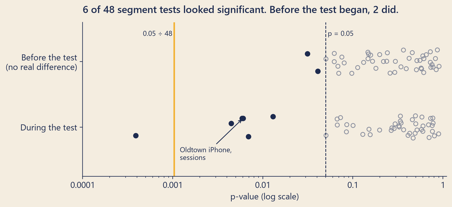
Mia could. Four cities, three platforms and four metrics made 48 tests. Of these, 6 came out “significant”. One of them looked like a headline:
Oldtown iPhone users opened the app 5.4% less often with the new prices (p = 0.006).
It is easy to build a story on that: Oldtown customers watch their money, and the new prices scared them away. But as the Prologue said, a story that fits is not the same as a story that is true.
Why it happens
Each test has a 5% chance of a false positive. Ask 48 questions of pure noise, and you should expect about 2.4 false positives. This is the multiple comparisons problem: the more tests you run, the more false positives you collect, even when each test is done correctly.
Mia found three reasons to doubt the Oldtown story.
Over the whole test, sessions per user barely moved: −0.5%, p = 0.411.
In the two weeks before the test, nobody had seen a new price. Yet Oldtown iPhone users in group B already opened the app 4.2% less often than those in group A (p = 0.062). By chance, the split had put slightly less active people into that small B group.
Mia ran all 48 tests again on those two weeks. There, every true difference is zero, yet 2 came out “significant”.
Show the code
rng_jitter = np.random.default_rng(7)fig, ax = bk.figure(8, 3.6)rows = [("Before the test\n(no real difference)", seg_pre, 1), ("During the test", seg, 0)]for label, frame, y in rows: p = frame.p.to_numpy() hit = p <0.05 yy = y + rng_jitter.uniform(-0.18, 0.18, len(frame)) ax.scatter(p[~hit], yy[~hit], s=28, facecolor="none", edgecolor=bk.MUTED, lw=1) ax.scatter(p[hit], yy[hit], s=36, color=bk.INK)if frame is seg: story_y = yy[seg.index.get_loc(story.name)]ax.axvline(0.05, color=bk.INK, ls="--", lw=1)ax.axvline(bonferroni, color=bk.MUSTARD, lw=2)ax.text(0.05, 1.42, " p = 0.05", fontsize=9, va="center")ax.text(bonferroni, 1.42, f"0.05 ÷ {n_tests} ", fontsize=9, va="center", ha="right")ax.annotate("Oldtown iPhone,\nsessions", xy=(story.p, story_y), xytext=(0.0012, -0.5), arrowprops=dict(arrowstyle="->", color=bk.INK), fontsize=9)ax.set_xscale("log")ax.set_xlim(1e-4, 1.1)ax.xaxis.set_major_formatter(mticker.FuncFormatter(lambda v, _: f"{v:g}"))ax.set_ylim(-0.75, 1.6)ax.set_yticks([0, 1], [rows[1][0], rows[0][0]])ax.grid(False)ax.set_xlabel("p-value (log scale)")ax.set_title(f"{n_sig} of {n_tests} segment tests looked significant. "f"Before the test began, {n_sig_pre} did.")plt.show()
Figure 2: Each dot is one segment test (city × platform × metric). Dots left of the dashed line have p below 0.05. The solid line is a stricter level, explained below.
How to catch it, and what to do
First, count the tests, including the ones nobody wrote down. Then correct for the count, in one of two ways.
The family-wise error rate (FWER) is the chance of at least one false positive among all the tests. Bonferroni controls it by dividing alpha by the number of tests: 0.05 ÷ 48 ≈ 0.0010. Holm is a step-by-step version with the same promise.
The false discovery rate (FDR) is the expected share of false positives among the results you call significant. The Benjamini–Hochberg method controls it. It is less strict and suits a first screen of leads you will check again.
Holm kept 1 result, and so did Benjamini–Hochberg: drinks per user for Oldtown iPhone users, down 9.7%. Drinks per user also fell clearly over the whole test (−5.2%, p < 0.001). Trust the whole-test number for the size: the biggest of 48 results is usually too big, because luck helped push it to the top.
The best fix comes before the test: one primary metric (Chapter 20), here revenue per user. Treat every other result, and every segment, as a hypothesis to check in a new test, not a finding. Orders per user, in Clue 3, passes this check: even with Holm’s stricter line for four tests, its p-value is small enough (p = 0.012 against 0.017).
NoteUnder the hood
With \(m\) independent tests and no real effects, the chance of at least one false positive is
\[1 - (1 - \alpha)^m.\]
With \(\alpha = 0.05\) and Mia’s 48 tests, that is 0.91.
Bonferroni: reject test \(i\) if \(p_i \le \alpha / m\). This keeps FWER \(\le \alpha\) for any dependence between tests.
Holm: sort the p-values, \(p_{(1)} \le p_{(2)} \le \dots \le p_{(m)}\). Reject them in order while \(p_{(j)} \le \alpha / (m - j + 1)\), and stop at the first one that fails. FWER \(\le \alpha\), again for any dependence.
Benjamini–Hochberg: find the largest \(k\) with \(p_{(k)} \le \frac{k}{m}\alpha\), and reject the \(k\) smallest p-values. This keeps \(\text{FDR} = E\left[\frac{V}{\max(R, 1)}\right] \le \alpha\), where \(V\) is the number of false rejections and \(R\) the number of all rejections. The proof needs the tests to be independent or positively related. Here the dependence is between the four related metrics inside each segment. Benjamini–Hochberg works well with this in practice; the stricter Benjamini–Yekutieli version covers any dependence.
Lie 3 · A coin that was not fair
What it looked like at Steep
Mia had learned to check the split before reading any result; it was in her plan for checkout_v2 (Chapter 20). An older test from July, checkout_redirect, shows why. Half of the users were meant to reach checkout through a new payment page, by way of a redirect: the app sends the user through an extra web page first.
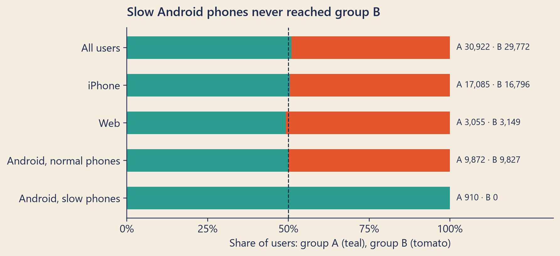
The result looked good. Conversion, the share of users who ordered, was up +2.1% in group B, with p < 0.001. Then Mia counted the users. Group A had 30,922. Group B had 29,772, which is 49.05% of the total.
That looks close to half. It is not close enough. With 60,694 users, a fair coin almost never lands that far from 50%. The chance is about 1 in 330,000.
Show the code
groups = [ ("All users", redirect), ("iPhone", redirect[redirect.platform =="ios"]), ("Web", redirect[redirect.platform =="web"]), ("Android, normal phones", redirect[(redirect.platform =="android") &~redirect.slow_device]), ("Android, slow phones", redirect[redirect.slow_device]),]fig, ax = bk.figure(8, 3.6)for row, (label, frame) inenumerate(reversed(groups)): n_a =int((frame.variant =="control").sum()) n_b =int((frame.variant =="treatment").sum()) share_a = n_a / (n_a + n_b) ax.barh(row, share_a, color=bk.TEAL, height=0.6) ax.barh(row, 1- share_a, left=share_a, color=bk.TOMATO, height=0.6) ax.text(1.02, row, f"A {n_a:,} · B {n_b:,}", va="center", fontsize=9)ax.axvline(0.5, color=bk.INK, ls="--", lw=1)ax.set_yticks(range(len(groups)), [label for label, _ inreversed(groups)])ax.xaxis.set_major_formatter(mticker.PercentFormatter(1.0))ax.set_xlim(0, 1.32)ax.set_xticks([0, 0.25, 0.5, 0.75, 1])ax.grid(False)ax.set_xlabel("Share of users: group A (teal), group B (tomato)")ax.set_title("Slow Android phones never reached group B")plt.show()
Figure 3: The split between the groups in checkout_redirect, by type of user. The planned split was 50/50.
Why it happens
Sample ratio mismatch (SRM) means the split is further from the plan than chance allows. Random assignment makes the groups alike only if every assigned user is counted. If some users go missing from one group only, the groups are no longer alike.
Mia split the count by platform. iPhone and web users were split fairly. Android users were not: group B had only 47.7% of them (p < 0.001). Among slow Android phones, group A had 910 users and group B had 0.
The redirect was too slow for slow phones. They timed out before the app could log their group, so they vanished from group B but not from group A. Slow phones are also where checkout is hardest. Group A kept the customers least likely to order, and group B lost them. Group B looked better because it had easier customers, not because the new page was better.
So Mia compared like with like: users with normal phones, in both groups. This is fair because a phone is slow or fast before the test begins. The test cannot change it. Now the split was fine (p = 0.326), and the lift was +0.2%, with p = 0.736. The win was gone. What was left was a bug: the redirect breaks checkout on slow phones.
How to catch it, and what to do
Check for SRM before you read any result. The check is a chi-square test: it compares the user counts with the planned split and gives a p-value for the gap. Many teams use a stricter line for SRM, p below 0.001. The check runs on every test, and real SRM bugs give far smaller p-values.
If the check fails, do not read the result, and do not “fix” it by weighting the groups back to 50/50: weights cannot bring back missing people. Find out where they went. Common causes are redirects, crashes, bots, logging that fails in one group, and filters on something the treatment can change.
Try it: the SRM checker
The checker starts with the numbers from checkout_redirect. Try dividing both counts by 100: the share in B stays the same, but the alarm goes away. A 49/51 split is alarming for sixty thousand users and normal for six hundred.
viewof srmInput = Inputs.form({a: Inputs.number({label:"Users in group A",value: srmDefault.control,min:0,step:1}),b: Inputs.number({label:"Users in group B",value: srmDefault.treatment,min:0,step:1}),share: Inputs.range([0.05,0.95], {label:"Planned share in B",value:0.5,step:0.05})})
Show the code
srmReadout = {const {a, b, share} = srmInput;if (!(a >0&& b >0)) returnhtml`<p>Enter two positive counts.</p>`;const total = a + b;const expectA = total * (1- share), expectB = total * share;const chi2 = (a - expectA) **2/ expectA + (b - expectB) **2/ expectB;const p =twoSidedP(Math.sqrt(chi2));// chi-square with 1 degree of freedomconst shown = p <1e-6?"< 0.000001": p <0.001? p.toExponential(1) : p.toFixed(3);const verdict = p <0.001?"Sample ratio mismatch. Do not read the results. Find out where the missing users went.": p <0.05?"A warning sign, not proof. Look for a cause before you trust the result.":"No sign of a mismatch. This does not prove the split is perfect; it only finds no evidence against it.";returnhtml`<p>Share in B: <strong>${(100* b / total).toFixed(2)}%</strong> (planned ${(100* share).toFixed(0)}%). Chi-square = <strong>${chi2.toFixed(2)}</strong>, p = <strong>${shown}</strong>.</p> <p><strong>${verdict}</strong></p>`;}
NoteUnder the hood
With \(N\) users in total and a planned share \(s\) for group B, the expected counts are \(E_A = N(1-s)\) and \(E_B = Ns\). The chi-square statistic adds up the squared gaps:
where \(O_A\) and \(O_B\) are the observed counts. With two groups it has one degree of freedom, so the p-value is \(P(\chi^2_1 > \chi^2)\), which equals the two-sided normal p-value of \(\sqrt{\chi^2}\).
Lie 4 · The shine wears off
What it looked like at Steep
In June, Steep tested home_v2, a new home screen with a one-tap “order again” button, for four weeks. Over the whole test, orders per user rose +4.0% (p < 0.001).
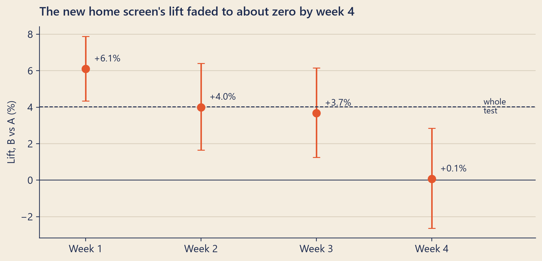
Mia asked how the lift changed as users got used to the new screen. She measured orders per user-day (one user for one day), by weeks since each user’s first exposure, the first day they saw it.
Show the code
fig, ax = bk.figure(8, 3.8)ax.errorbar(weekly.week, 100* weekly.lift, yerr=[100* (weekly.lift - weekly.lo), 100* (weekly.hi - weekly.lift)], fmt="o", color=bk.TOMATO, ecolor=bk.TOMATO, ms=8, capsize=4, lw=1.6)for row in weekly.itertuples(): ax.annotate(pct(row.lift), (row.week, 100* row.lift), xytext=(9, 6), textcoords="offset points", va="bottom", fontsize=10)ax.axhline(0, color=bk.INK, lw=0.8)ax.axhline(100* home_pooled_lift, color=bk.INK, ls="--", lw=1)ax.text(4.45, 100* home_pooled_lift, "whole\ntest", va="center", fontsize=9)ax.set_xticks(weekly.week, [f"Week {k}"for k in weekly.week])ax.set_xlim(0.6, 4.9)ax.set_ylabel("Lift, B vs A (%)")ax.set_title("The new home screen's lift faded to about zero by week 4")plt.show()
Figure 4: Lift in orders per user-day for home_v2, by week since each user first saw the new home screen. Bars show 95% intervals. The dashed line is the whole test, in the same unit.
Week by week, the lift was +6.1%, +4.0%, +3.7% and +0.1%. The week-4 interval runs from −2.6% to +2.8%. The dashed line is the whole test in the same unit, per user-day: +4.0%.
Why it happens
This is the novelty effect from Chapter 20: people tap a new button to see what it does, and a few weeks later it is an ordinary button. (The opposite, change aversion, also happens.) Either way, the early weeks are a poor guide to the long run.
Users joined on different days, but the test ended on one date, so only early joiners have a fourth week. Every user has a first week, so a whole-test average leans toward the shiny part. It also means the bars hold different people (65,947 users in week 1, 47,065 in week 4).
How to catch it, and what to do
Plot the lift by weeks since first exposure, not by calendar date, and run until that curve goes flat: at least two full weeks, so that every weekday appears twice.
Report the settled effect with its interval: for home_v2, close to zero. The redesign may still be worth keeping, but not for a lasting +4.0% in orders.
Lie 5 · Groups that share couriers
What it could look like at Steep
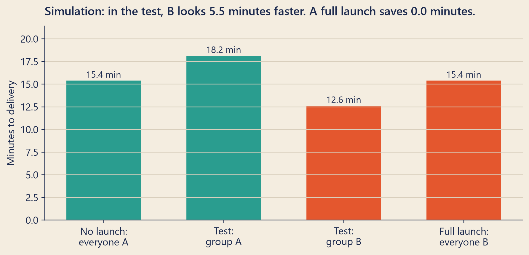
Steep never ran this test, so imagine it: “priority delivery”. Orders in group B jump to the front of the courier queue. Delivery times in group B fall, and the test shows a big win.
But couriers are shared. Every courier who takes a B order first is not taking an A order. Group B is faster partly because group A is slower.
Mia built a small simulation, not Steep data: one busy city, 30 couriers, and made-up orders and trip times. The same orders arrive in every version; only the priority changes.
Show the code
fig, ax = bk.figure(8, 3.8)colors = [bk.TEAL, bk.TEAL, bk.TOMATO, bk.TOMATO]bars = ax.bar(list(sim), list(sim.values()), color=colors, width=0.62)for bar, value inzip(bars, sim.values()): ax.text(bar.get_x() + bar.get_width() /2, value +0.3, f"{value:.1f} min", ha="center", fontsize=10)ax.set_ylabel("Minutes to delivery")ax.set_ylim(0, max(sim.values()) *1.18)ax.set_title(f"Simulation: in the test, B looks {test_gap:.1f} minutes faster. "f"A full launch saves {launch_gain:.1f} minutes.")plt.show()
Figure 5: SIMULATION, not Steep data. Average minutes from order to delivery in one busy city with shared couriers.
In the test, B looks 5.5 minutes faster than A. But launch it to everyone, and the average is 15.4 minutes, the same as with no launch. When everyone has priority, nobody does: priority changes the order of the queue, not the speed of the couriers.
Why it happens
Interference (or spillover) happens when one user’s group changes another user’s result. A simple A/B test assumes there is none: my result should depend only on my own group. Shared resources break that rule. At Steep, they include couriers, store kitchens and limited stock.
How to catch it, and what to do
Ask of every test: do the two groups compete for anything, such as couriers, stock or kitchen time?
Randomise a bigger unit, so that A and B no longer share, such as whole cities. But four cities give only four data points.
Or run a switchback test: the whole city switches between A and B in time slots, such as hours, in a random order. Compare A hours with B hours, counting each hour as one observation.
Lie 6 · Counting orders instead of people
What it looked like at Steep
Priya’s dashboard had one more number: average order value (AOV), revenue per order. It was up +1.5%, from $11.97 to $12.15, and its test treated each of the 87,056 orders as one independent observation.
AOV is a ratio metric, one total divided by another, and it hides two traps.
The first trap is the bottom number. A ratio can rise because its bottom number falls. AOV rose because each drink cost more, while people placed fewer orders. Revenue per user, the number that pays the bills, did not move.
The second trap is the unit. The test assigned users to groups, not orders. A user who orders five times brings five related orders into the same group: the same person, with the same habits. A test that counts them as five independent facts usually gets too narrow an interval, because a person’s orders tend to be alike.
How to catch it, and what to do
Analyse at the level you randomised: the user. There are two standard ways.
The delta method is a formula that gives the right uncertainty for a ratio, using each user’s totals.
A user-level bootstrap resamples people, not orders: within each group, draw users at random with replacement (the same person can be picked twice), keep all their orders, recompute the ratio, and repeat a thousand times.
Mia tried all three on the real price-test data. The standard error (Chapter 17) is the usual size of the random wobble in an estimate.
Method
Standard error of the AOV difference
Naive: each order is independent
$0.0332
Delta method: users are independent
$0.0331
Bootstrap: resample users
$0.0334
They agree. Here, Steep’s data makes the mistake harmless: what a person spends on one order says almost nothing about their next one. Real customers usually have stronger habits.
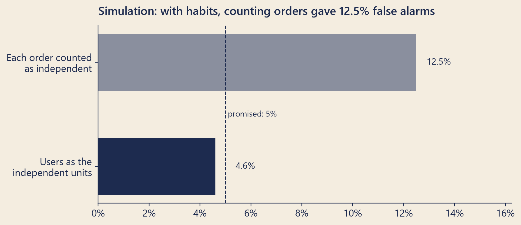
So Mia ran a simulation. She kept the real users and their real order counts, but gave each user a made-up habit, so that some people always spend more per order than others. Then she ran 1,000 A/A splits of these users and counted the false alarms.
Show the code
fig, ax = bk.figure(8, 3.4)labels = ["Each order counted\nas independent", "Users as the\nindependent units"]values = [fpr_naive, fpr_user]bars = ax.barh(labels, values, color=[bk.MUTED, bk.INK], height=0.55)for bar, value inzip(bars, values): ax.text(max(value, 0.05) +0.004, bar.get_y() + bar.get_height() /2, bk.fmt_pct(value), va="center", fontsize=10)ax.axvline(0.05, color=bk.INK, ls="--", lw=1)ax.text(0.05, 0.5, " promised: 5%", fontsize=9, va="center", transform=ax.get_xaxis_transform())ax.invert_yaxis()ax.xaxis.set_major_formatter(mticker.PercentFormatter(1.0, decimals=0))ax.set_xlim(0, max(values) *1.3)ax.grid(False)ax.set_title(f"Simulation: with habits, counting orders gave {bk.fmt_pct(fpr_naive)} false alarms")plt.show()
Figure 6: SIMULATION. Real order counts from the price test, with made-up ordering habits. False alarms in 1,000 A/A splits.
With habits, the naive method raised 12.5% false alarms instead of 5%. The user-level method stayed at 4.6%.
NoteUnder the hood
In one group, let user \(i\) have revenue \(Y_i\) and orders \(X_i\), for \(n\) users. AOV is the ratio \(R = \bar Y / \bar X\). The naive method treats all \(\sum X_i\) orders as independent, so its variance is \(s^2_{\text{order}} / \sum X_i\).
The delta method treats users as independent. A first-order Taylor expansion of \(\bar Y / \bar X\) gives
where \(s_Y^2\), \(s_X^2\) and \(s_{XY}\) are the variances and covariance of the per-user totals.
If orders from the same user share a correlation \(\rho\), the naive variance is too small by a factor of roughly \(1 + (\bar m - 1)\rho\), where \(\bar m = \sum X_i^2 / \sum X_i\). In the price test, \(\bar m\) is about 2.96. In Steep’s data, \(\rho\) is close to 0, so the factor is close to 1. The simulation uses \(\rho\) = 0.3, so the naive standard error is too small by a factor of about 1.26: its line at 1.96 is really at about 1.55, which noise crosses 12.0% of the time, as the simulation found.
The lift intervals in this chapter use the same idea: \(\operatorname{Var}(\bar B/\bar A) \approx \frac{s_B^2}{n_B \bar A^2} + \frac{\bar B^2 s_A^2}{n_A \bar A^4}\).
Lie 7 · One customer decides
What it could have looked like at Steep
Steep’s experiment platform keeps corporate accounts out of every test. On 11 August, during the price test, one corporate account placed a single order of 400 drinks, worth $2,636.50. What if it had been in the test?
This is a what-if, not what happened: Mia added that order to one group in a copy of the data and reran the test, with and without a cap (explained below).
Revenue per user
Lift
p-value
Lift, capped
p-value, capped
As measured
−0.6%
0.489
−0.6%
0.493
What-if: order in B
−0.1%
0.903
−0.6%
0.508
What-if: order in A
−1.1%
0.276
−0.6%
0.479
One order out of 87,057 moves the result by about 0.5 points either way, almost as much as the revenue lift the test measured, −0.6%. An outlier like this is far from the rest, and a mean adds up every value, so one huge value can move it a lot, more so in a small test.
How to catch it, and what to do
Decide before the test how you will treat extreme values. A common choice is to winsorize: replace every value above a cap with the cap itself. Set the cap from data you had before the test. Mia used the 99.9th percentile of revenue per user in the two weeks before (the value that 99.9% of users are below): $123.71.
With the cap, all three rows say the same thing: −0.6%. A capped test measures the effect on revenue with very large values trimmed. If big customers matter, look at them separately.
Look at the largest values by hand.
Do not remove outliers after you see the result. If you choose what to remove once you know which way it pushes, you will push the answer toward the one you hoped for.
The seven lies on one screen
Lie
Symptom
The check
The fix
1 · Peeking
A winner declared before the planned end
Compare the decision date with the planned end; plot p by day
Fixed horizon, read once; or sequential tests (Ch 22)
2 · Too many questions
A surprising segment “finding”
Count every test; apply Holm or Benjamini–Hochberg
One primary metric chosen in advance; segments become new hypotheses
3 · Unfair coin (SRM)
User counts far from the planned split
Chi-square test on counts, also by platform and day
Stop; find the missing users; never reweight
4 · Novelty
A big early lift that fades
Lift by days since first exposure
Run longer; report the settled effect
5 · Interference
Groups share couriers, stock or money
Ask what A and B compete for
Randomise cities or time slots (switchback)
6 · Wrong unit
A ratio analysed per order, not per user
Compare naive and user-level errors
Delta method or user-level bootstrap
7 · Outliers
One huge value moves the result
Look at the largest values; recompute with a cap
A cap (winsorize) set before the test
Common traps
“Not significant” is not “no effect”. Revenue per user was not significant, but its interval runs from −2.4% to +1.1%. That range includes changes Dana would care about.
Changing the question after the test. Reporting AOV instead of the planned revenue per user, because AOV went up, is a quiet form of Lie 2.
TipAudit Instinct · Plan before fieldwork
Auditors plan before they look. Before they open a single invoice, they set materiality: how large an error must be to matter. They define the population, the records in scope. And they write the sampling plan: how many items, chosen how. They do this first, so that the results cannot bend the plan.
Then, before they sample, they reconcile the population. The list they sample from must agree with the ledger total. A sample from an incomplete list proves nothing about the missing part.
An A/B test needs the same discipline. Pre-registration (Chapter 20) is materiality and the sampling plan in a new job, and the SRM check is the population reconciliation: before you trust what the groups did, prove that they hold everyone they should.
NoteInterview Corner
1. Why does peeking inflate the false-positive rate?
NoteA model answer
A 0.05 line promises 5% false positives for one look at a fixed time. With no real effect, the p-value wanders, so stopping at the first value below 0.05 gives many chances to cross: about 22% with 14 equal daily looks, and close to 100% with no limit. Use a fixed horizon or a sequential method (Chapter 22).
2. How do you detect and handle a sample ratio mismatch?
NoteA model answer
Before reading any result, run a chi-square test of the user counts against the planned split, with a strict alarm level such as 0.001, also by platform and by day. If it fails, do not trust or reweight the result. Find the cause, fix it, and rerun.
3. A test shows a +3% lift in week 1 but +0.5% in week 3. What do you report?
NoteA model answer
Report the settled effect, about +0.5%, with its interval and whether it includes zero. Call the early lift a likely novelty effect, and plot the lift by days since first exposure to check that it has stopped falling; if not, run longer.
Reported change: −12.0% orders, the week of 7 September compared with the week before (CEO dashboard).
Explained so far: 12.0 of the 12 points.
Piece
Points
Where
Tracking bug: Apple Pay orders on iOS 3.2.0 sent no order_completed event
7.0
Chapter 15
Rainy week before, dry week of the drop
3.4
Chapter 16
Normal weekly growth, which pushes the other way
−0.3
Chapter 16
What is left: orders below the recipe’s prediction (the price rise)
1.9
This chapter
Total
12.0
Chapter 16’s recipe predicted −3.1% (normal growth plus the real rain). Completed orders (finance’s definition, final statuses; see Chapter 1) came in at −5.0%: 1.9 points lower. The price test, measured separately, agrees: 2.1% fewer orders, on a week the recipe expected at 96.9% of the week before, is about 2.1 points of the 12 (interval 0.5 to 3.7).
Suspects: the 5% price rise for everyone on 7 September (price_up_5): proved (this chapter).
Ruled out: the matcha menu (Chapter 4); every stop on the data’s journey after the app (Chapters 8–14); Priya’s day-3 “win” for revenue per user, a product of peeking (this chapter).
Open questions: Did Riverside’s new delivery fee, in force since 5 October, cost orders (Chapter 23)? How should Mia tell the board of directors (Chapter 24)?
New evidence: the full 14-day price test, read once.
Recap
Plan the question, the primary metric, the sample size and the end date before the test. Then read the result once, at the end.
Check that the split was fair before you read the result: SRM first, then the effect.
Analyse at the level you randomised, for long enough, with a rule for extreme values, and with a count of every question you asked.
English
中文
peeking
偷看 / 提前看结果
false positive
假阳性
A/A test
A/A 测试
multiple comparisons
多重比较
family-wise error rate (FWER)
族错误率
false discovery rate (FDR)
错误发现率
sample ratio mismatch (SRM)
样本比例失衡
novelty effect
新奇效应
interference
干扰 / 溢出效应
switchback test
轮转实验
ratio metric
比率指标
delta method
Delta 方法
winsorize
缩尾
pre-registration
预注册
guardrail metric
护栏指标
Further reading
Kohavi, R., Tang, D., & Xu, Y. (2020). Trustworthy Online Controlled Experiments. Cambridge University Press. DOI
Johari, R., Koomen, P., Pekelis, L., & Walsh, D. (2017). Peeking at A/B Tests. Proceedings of the 23rd ACM SIGKDD International Conference on Knowledge Discovery and Data Mining. DOI
Fabijan, A., Gupchup, J., Gupta, S., Omhover, J., Qin, W., Vermeer, L., & Dmitriev, P. (2019). Diagnosing Sample Ratio Mismatch in Online Controlled Experiments. Proceedings of the 25th ACM SIGKDD International Conference on Knowledge Discovery & Data Mining. DOI
Holm, S. (1979). A Simple Sequentially Rejective Multiple Test Procedure. Scandinavian Journal of Statistics, 6, 65–70.
Benjamini, Y., & Hochberg, Y. (1995). Controlling the False Discovery Rate: A Practical and Powerful Approach to Multiple Testing. Journal of the Royal Statistical Society: Series B, 57(1), 289–300. DOI
Deng, A., Knoblich, U., & Lu, J. (2018). Applying the Delta Method in Metric Analytics. Proceedings of the 24th ACM SIGKDD International Conference on Knowledge Discovery & Data Mining. DOI
Bojinov, I., Simchi-Levi, D., & Zhao, J. (2023). Design and Analysis of Switchback Experiments. Management Science, 69(7). DOI