On Wednesday, Dana came to Mia’s desk with yesterday’s note in her hand.
“‘The weekly numbers cannot tell a 2% drop in orders from noise. Suspect: the price rise,’” she read. She put the note down. “Two things bother me. We had 43,153 orders that week, and you still cannot tell. And Priya tested those prices in August, and her test said they were a win. How can so much data say so little? And how can a test say ‘win’ about a change that may have cost us orders?”
“Both questions have the same answer,” Mia said. “A test can only see a change that is big enough for its size. Priya’s test was judged on revenue per user, after three days. And a week of totals is a smaller net than it looks.”
“A net?”
Mia turned her notebook back three weeks. “Let me show you how I planned the checkout test. Then both will make sense.”
Friday, 18 September. At the end of Mia’s first week, Priya Nair, the product manager, came to her desk. On her laptop were two checkout screens. The old checkout took three steps. The new one, checkout_v2, put everything on one page.
“I want to test it,” Priya said. “Half the users get the new page, half keep the old one. Can we start Monday?”
“We can,” Mia said. “But first: how many users do we need to see it?”
Priya blinked. “To see what?”
“The change you hope for. How big is it?”
“Big, I hope. Five percent more customers ordering?”
“And the smallest change you would still want to know about?”
Priya thought. “One percent. One percent more customers ordering is a lot of tea.”
Mia wrote both numbers in her notebook. Then she opened the data.
ImportantThe big idea
Decide before the test how small a change you need to see, and collect enough data to see it.
Two nets
Look at the picture at the top of this chapter. Two nets hang over the same pond, full of the same small fish. The small net has wide holes, and the fish slip through. The big net has fine mesh, and it holds them.
A test is a net, and real effects are the fish. Whether you catch a small fish depends on the net, not only on the fish.
Power is the chance that a test catches a real effect of a given size: that it gives a significant result when the effect is really there (Chapter 18). Power belongs to one size of fish at a time. A net can have high power for big fish and low power for small ones.
The minimum detectable effect (MDE) is the smallest effect a test catches with the power you planned, usually 80%. Smaller effects can still be caught, only less often.
The sample size is the number of units in the test, here users. It sets the size of the net.
The order matters. First, you decide which fish you need to catch: the MDE. Then you build a net big enough to catch it most of the time. A test planned the other way round, by starting it and seeing what comes out, often turns out to be a small net.
What sets the size of the net
Five things decide how many users a test needs.
Noise. The more an outcome varies from user to user, the more users you need. For a yes-or-no outcome, such as “did this user order?”, the noise depends on the baseline: the rate before any change.
Effect size. How big a change you want to see: the MDE. Small effects need many users.
Alpha. A stricter line for false alarms (Chapter 18) needs more evidence.
Power. Catching the effect 90% of the time instead of 80% needs more users.
The split. For a fixed number of users, a 50/50 split gives the most power. With a 90/10 split, the same test needs about 2.8 times as many users.
Noise and effect size are the strongest dials, because of a square root. The noise in an average shrinks with the square root of the number of users (Chapter 17). So, roughly: users needed ≈ (noise ÷ effect)², times a number set by alpha and power. Halve the effect, and you need four times the users. Halve the noise (Chapter 22 shows one way), and you need a quarter. Twice the users does not halve the MDE: it shrinks it by about 30%.
Mia’s plan
Priya’s idea is an A/B test. Users are split at random into group A, which keeps the old checkout, and group B, which gets the new one. Then the two groups are compared (Chapter 20 follows one from start to end). The lift is how much higher B’s number is than A’s, as a share of A’s.
The test’s main number would be conversion: the share of users in the test who complete at least one order during it. Each customer who opens the app during the test joins it once, at random, and stays in the same group. Corporate accounts are left out, as in every Steep test.
To plan, Mia needed two facts about Steep: how many users come, and how many of them order. She used the last whole weeks she had, up to Sunday 13 September. In the two weeks up to that day, Steep had 66,794 app users (customers who opened the app), and 67.0% of them ordered at least once. That is the baseline. Those were the two weeks of the case, one rainy and one with new prices, so Mia checked the two weeks before them (17 to 30 August): conversion was 67.4%, close enough for a plan. All lifts in this chapter are relative: a 2% lift on a conversion of 67.0% gives 68.3%, not 69.0%.
A longer test changes both numbers. More users come, but slowly, because many frequent customers come every week anyway. And conversion rises, because each user has more days to order. So Mia made a table. For a test of one to six weeks, it shows how many users come, how many order, and the smallest lift the test could see with 80% power at alpha 0.05. The table assumes the lift keeps the same size as conversion grows. Often it shrinks, so longer tests gain less than the table shows.
Weeks
App users
Conversion
Smallest lift seen (MDE)
Power for a 2% lift
1
53,701
54.8%
2.19%
72%
2
66,794
67.0%
1.52%
96%
3
72,081
74.1%
1.23%
>99%
4
74,964
78.7%
1.06%
>99%
5
76,662
82.0%
0.94%
>99%
6
77,813
84.3%
0.86%
>99%
Priya read it twice. “One percent needs five weeks?”
“Five whole weeks, to 25 October. And 2% needs two.”
“Five weeks of half our customers on the old checkout, if the new one is better,” Priya said. “And the payments team waits all that time to move on.” She looked at the table again. “What do we lose with two weeks?”
“We see a lift of 2% almost every time: power 96%. A lift of 1.5%, 79% of the time. A lift of 1%, only 45%: close to a coin flip.”
Priya nodded. “Two weeks. If the truth is 1%, we may miss it. I can accept that, if we write it down.”
So the plan used an MDE of 2%. Ideally, the MDE is no bigger than the smallest effect that matters. Here it was twice as big, and both of them knew it.
At the two-week conversion of 67.0%, a 2% lift (to 68.3%) needs about 19,100 users in each group. A shorter test needs more, because its users have had less time to order, so its conversion is lower. Mia checked day by day:
Test length
App users per group
Conversion
Users needed per group
Enough?
7 days
26,850
54.8%
32,310
No
9 days
29,548
59.1%
26,991
Yes: the first day
14 days
33,397
67.0%
19,121
Yes
Day 9 was the first day with enough users. Mia rounded up to whole weeks: 14 days. Rounding up has a bonus: with two whole weeks of users, the test can really see lifts down to 1.52%, not only 2%.
Why whole weeks? Steep’s orders follow a weekly pattern: Fridays and Saturdays are busy, and Mondays are quiet (Chapter 16). The people who order on a Saturday may not behave like the people who order on a Monday. A test that runs 9 days has two of some weekdays and one of others, so it is not a fair picture of a normal week. Whole weeks give every weekday the same weight. Two weeks also let Mia compare the first week with the second, to check that the effect does not fade as the new page stops being new (Chapter 20 checks this novelty effect).
Mia wrote the plan on one page and sent it to Priya and Theo before the test began.
Mia’s plan for checkout_v2, written Friday 18 September
Question
Does a one-page checkout raise conversion?
Who
Every customer who opens the app during the test (not corporate accounts), split 50/50 at random by user
Primary metric
Conversion: share of users with at least one completed order during the test
Baseline
67.0% (two weeks to 13 September)
Smallest lift to see (MDE)
+2% relative: 67.0% → 68.3%
Alpha · power
0.05, two-sided · 80%
Users needed
About 19,100 per group at the two-week conversion; enough users from day 9
Duration
Two whole weeks: Monday 21 September to Sunday 4 October
Read the result
Once, after the last day
Known limit
Power for a 1.5% lift: 79%; for 1%: 45%
Try it: the sample-size calculator
Use Steep’s real traffic from the two weeks to 13 September and the weeks before. Choose the smallest lift you want to see, and the calculator finds the first day with enough users, then rounds up to whole weeks. Try 1%, try a 90/10 split, and try asking for 95% power.
calcReadout = {const {first, weeks, runWeeks} = calcPlan;const fmt = (n) =>Math.round(n).toLocaleString("en-US");const pctf = (x) => (100* x).toFixed(1) +"%";const MONTHS = ["Jan","Feb","Mar","Apr","May","Jun","Jul","Aug","Sep","Oct","Nov","Dec"];const DAYS = ["Sun","Mon","Tue","Wed","Thu","Fri","Sat"];const [y, mo, d] = calcFacts.start.split("-").map(Number);const show = (date) =>`${DAYS[date.getDay()]}${date.getDate()}${MONTHS[date.getMonth()]}`;const start =newDate(y, mo -1, d);const end =newDate(y, mo -1, d +7* (runWeeks ||0) -1);const head = first?html`<p>Enough users after <strong>${first.days} day${first.days>1?"s":""}</strong>:${fmt(first.users)} users had come (both groups), and ${fmt(first.need)} were needed (${fmt(first.need/2)} per group) at that day's conversion of${pctf(first.conversion)}.</p> <p><strong>Run ${runWeeks} whole week${runWeeks >1?"s":""}</strong>: ${show(start)} to ${show(end)}.</p>`:html`<p><strong>Six weeks of Steep's traffic are not enough for this plan.</strong> Accept a bigger lift, less power or a 50/50 split, or find a way to reduce the noise (Chapter 22).</p>`;returnhtml`${head} <div class="table-responsive"><table class="table table-sm" style="font-size:0.8rem"> <thead><tr><th>Wk</th><th>Users</th><th>Conv.</th><th>Needed</th><th>Power</th></tr></thead> <tbody>${weeks.map((w) =>html`<tr><td>${w.weeks}</td><td>${fmt(w.users)}</td> <td>${pctf(w.conversion)}</td><td>${fmt(w.need)}</td> <td>${w.power>=0.995?">99%": (100* w.power).toFixed(0) +"%"}</td></tr>`)}</tbody> </table></div> <p style="font-size:0.85rem">Wk = weeks of testing. Users and Needed count both groups together. Conv. is the share of users who ordered.</p>`;}
Show the code
calcChart = Plot.plot({width:Math.min(width,640),height:220,marginLeft:48,style: {background:"transparent",fontSize:"12px"},x: {type:"band",label:"Weeks of testing →"},y: {domain: [0,1],label:"↑ Power for your lift",tickFormat: (d) =>`${(100* d).toFixed(0)}%`},color: {domain: ["enough users","not enough"],range: ["#2a9d8f","#8a8f9e"],legend:true},marks: [ Plot.barY(calcPlan.weeks, {x:"weeks",y:"power",fill:"status"}), Plot.ruleY([calcSettings.power], {stroke:"#1d2b4f",strokeDasharray:"4,3"}), Plot.ruleY([0]) ]})
Show the code
functionnormCdf(z) {const x =Math.abs(z) /Math.SQRT2;const t =1/ (1+0.3275911* x);const tail = t * (0.254829592+ t * (-0.284496736+ t * (1.421413741+ t * (-1.453152027+ t *1.061405429)))) *Math.exp(-x * x) /2;return z >=0?1- tail : tail;}// Its inverse, by bisection: the z with normCdf(z) = q.functionnormInv(q) {let lo =-10, hi =10;for (let i =0; i <80; i++) {const mid = (lo + hi) /2;if (normCdf(mid) < q) lo = mid;else hi = mid; }return (lo + hi) /2;}
The dashed line is the power you asked for. Notice how slowly the users grow after two weeks, while the power still rises. Longer tests gain power here mostly because each user has more days to order.
Back to the price test
Back in Wednesday’s meeting, Dana had followed all of it. “So a test is a net,” she said. “How big was Priya’s net?”
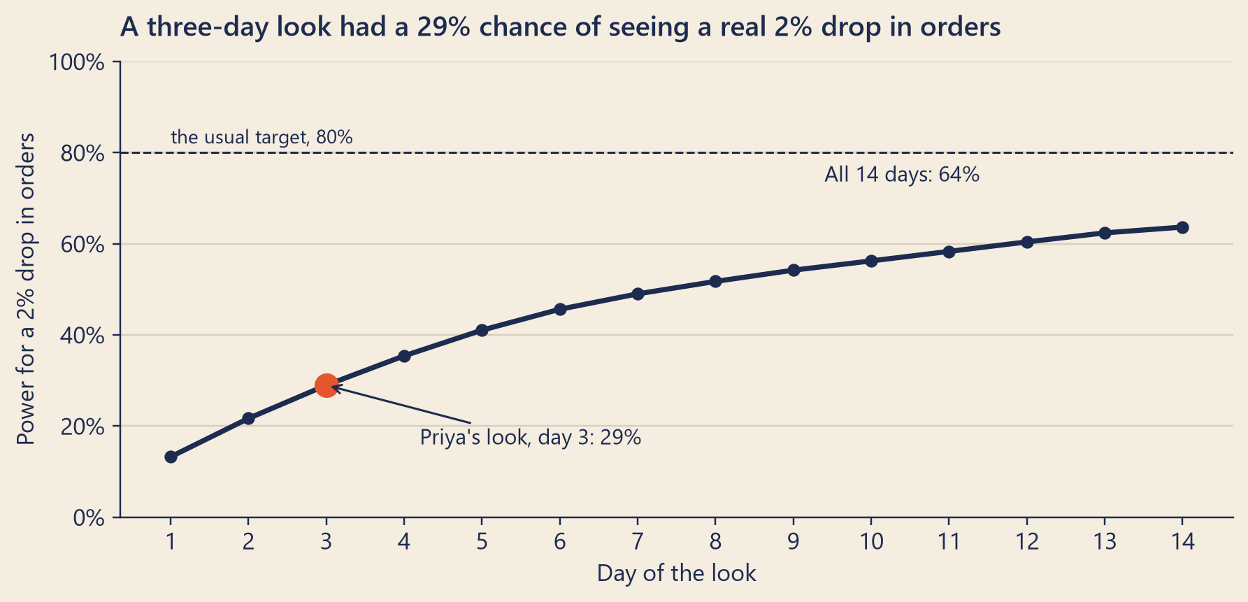
Mia did the same sums for price_up_5. Its main metric was revenue per user, but Dana’s question was about orders, and so was Mia’s suspect. So Mia asked: if the new prices really cut orders per user by 2%, what was the chance that a look after three days would show it?
She did not need the test’s result for this, only its size and its noise. By the end of day 3, 31,827 users had joined: about 15,900 per group. Each user in group A had placed 0.52 orders so far, on average, with a standard deviation of 0.66. So the noise was 1.27 times the mean. 56% of them had not ordered at all yet.
Show the code
fig, ax = bk.figure(8, 3.8)ax.plot(look.index, look.power, color=bk.INK, lw=2.4, marker="o", ms=5)ax.scatter([LOOK_DAY], [day3.power], s=110, color=bk.TOMATO, zorder=3)ax.annotate(f"Priya's look, day {LOOK_DAY}: {pct(day3.power, 0)}", (LOOK_DAY, day3.power), xytext=(LOOK_DAY +1.2, day3.power -0.13), arrowprops=dict(arrowstyle="->", color=bk.INK), fontsize=10)ax.annotate(f"All {n_days} days: {pct(day_end.power, 0)}", (n_days, day_end.power), xytext=(n_days -4.6, day_end.power +0.1), fontsize=10)ax.axhline(POWER, color=bk.INK, ls="--", lw=1)ax.text(1, POWER +0.02, "the usual target, 80%", fontsize=9)ax.set_ylim(0, 1)ax.yaxis.set_major_formatter(plt.FuncFormatter(lambda v, _: f"{100* v:.0f}%"))ax.set_xticks(range(1, n_days +1))ax.set_xlabel("Day of the look")ax.set_ylabel("Power for a 2% drop in orders")ax.set_title(f"A three-day look had a {pct(day3.power, 0)} chance of seeing a real 2% drop in orders")plt.show()
Figure 1: The power of a look at price_up_5 after each day: the chance that the test would show a real 2% drop in orders per user as significant (alpha 0.05, two-sided). Computed from the group sizes and group A’s noise, not from the result.
Here is the arithmetic. The standard error of the lift (Chapter 17) was about 1.27 × √(4 ÷ 31,827) ≈ 1.4 percentage points. A 2% drop is about 1.4 standard errors from zero. But to be significant, an estimate must be at least 1.96 × 1.4 ≈ 2.8 points from zero. So a three-day look would catch a real 2% drop only about 3 times in 10: its power was 29%. For 80% power, each group needed about 15.7 × (1.27 ÷ 0.02)² ≈ 63,000 users. That is the rule (noise ÷ effect)², and 15.7 is the number for alpha 0.05 and 80% power. Day 3 had about 15,900 per group. Even all 14 days gave only 64%. The test’s main metric was revenue, not orders.
“So the test could not see a 2% loss in orders,” Dana said.
“It could, sometimes. Usually it would not. A small net catches a small fish only with luck.”
“And it said ‘win’ about revenue, after three days.”
“Yes. That raises a different question,” Mia said. “When a small net does catch something, how much should you trust the catch? But first, your other question.”
Three nets for the same fish
Dana’s other question was about the weekly totals. Yesterday’s weekly test had only 33% power for a 2% drop in orders (Chapter 18). Next to the price test, the three nets look like this.
The net
Power for a real 2% drop in orders
Weekly totals: the week of the drop against the week before (Chapter 18)
33%
price_up_5, read after three days
29%
price_up_5, all 14 days
64%
All three are below the usual 80%. None of them was a reliable net for a 2% fish.
Why is a week of 43,153 orders such a small net? Because the noise in a weekly total does not come mainly from single orders. Counting luck alone moves a week of about 44,000 orders by only about 0.48% (for a count, chance alone gives a spread of about its square root). For the difference of two weeks, the spread grows by about 1.4 (the square root of 2), to about 0.7 points. With noise that small, the weekly test would catch a 2% drop 83% of the time. But real summer weeks missed the recipe by 1.07% (Chapter 18), and 1.07 × 1.4 ≈ 1.5 points. Whole weeks move together, pushed by things such as a local event, a holiday or one of Steep’s own tests. Comparing one week with another is a test of two weeks, not of tens of thousands of orders.
A randomised test gets around this. It splits users at random over the same days. Whatever moves a whole week moves both groups alike, and it cancels out when you compare them. What is left is the noise from one user to the next, and that shrinks as more users join. That is why the full 14-day test was the strongest of the three nets, and why Chapter 21 goes back to it.
The winner’s curse
Here is the trouble with a small net. When it does catch something, the catch looks bigger than the fish really is.
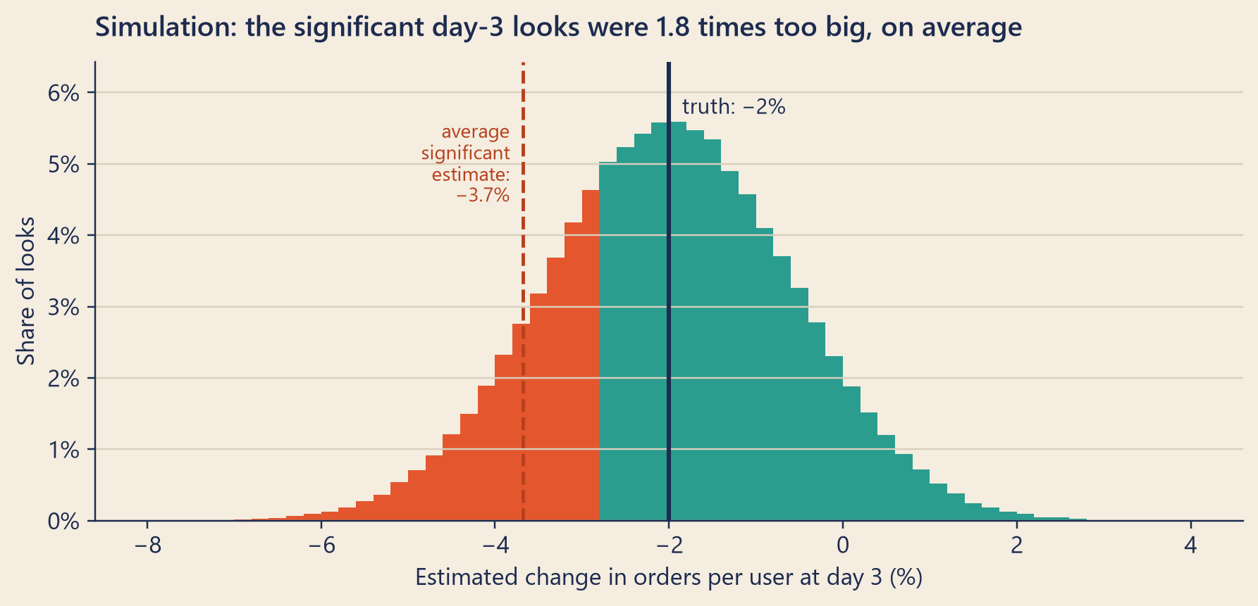
Mia ran a simulation of the day-3 look. Suppose the price rise really did cut orders per user by 2%. A three-day look measures that 2% with a lot of noise: its standard error was 1.4 percentage points (Chapter 17). She drew 200,000 such day-3 estimates and kept the ones that would have been called significant.
Show the code
fig, ax = bk.figure(8, 3.8)bins = np.arange(-8, 4.01, 0.2)heights, _ = np.histogram(100* est, bins=bins)centres = (bins[:-1] + bins[1:]) /2significant = np.abs(centres) >=100* lineax.bar(centres, heights / SIMS, width=0.2, color=np.where(significant, bk.TOMATO, bk.TEAL), lw=0)ax.axvline(-100* PRICE_CUT, color=bk.INK, lw=2)ax.axvline(-100* sig_size, color=bk.TOMATO_TEXT, lw=1.6, ls="--")top = heights.max() / SIMSax.text(-100* PRICE_CUT +0.15, top *1.02, f"truth: −{pct(PRICE_CUT, 0)}", fontsize=10)ax.text(-100* sig_size -0.15, top *0.8, f"average\nsignificant\nestimate:\n−{pct(sig_size)}", fontsize=9, ha="right", color=bk.TOMATO_TEXT)ax.yaxis.set_major_formatter(plt.FuncFormatter(lambda v, _: f"{100* v:.0f}%"))ax.set_ylim(0, top *1.15)ax.set_xlabel("Estimated change in orders per user at day 3 (%)")ax.set_ylabel("Share of looks")ax.set_title(f"Simulation: the significant day-3 looks were {exaggeration:.1f} times too big, on average")plt.show()
Figure 2: SIMULATION. 200,000 three-day looks at a true 2% drop in orders, each with the noise of the real day-3 look. Tomato bars would have been called significant.
Only 29% were significant, as the power said. To be significant, an estimate had to be at least 2.8% away from zero, which is further than the true 2%. So the significant estimates averaged 3.7% in size: 1.8 times the truth.
This is the winner’s curse. In an underpowered test (one with low power for the effects that matter), the results that pass the significance line are mostly the lucky ones, so they overstate the effect. A very few even point the wrong way: here, about 1 significant result in 760. That is for one look, planned for day 3. Looking every day gives luck many more chances, and Chapter 21 meets a wrong-way result in the price test’s very first day.
A test with enough power hardly suffers. Mia’s checkout plan had 79% power for a 1.5% lift. In the same kind of simulation, its significant results overstate a true 1.5% by only about 13%.
So when a small, early look shows a big significant result, expect the real effect to be smaller, and sometimes absent. Priya’s three-day win was about revenue per user, which is a little noisier than orders. Chapter 21 shows what happened to it when all 14 days came in.
Real, but big enough to matter?
A result can be statistically significant and still too small to care about. With enough users, a test can see very small changes. With six weeks of Steep’s traffic, the checkout test could have seen lifts as small as 0.9%. With ten times Steep’s users, two weeks could see lifts of about 0.5%. Real, yes. Worth a project? Not always.
This is the difference between statistical significance (data this far from zero would be rare if there were no effect) and practical significance (the effect is big enough to matter to the business). The second is a business question, not a statistics question. Priya answered it on 18 September: for her, 1% was the smallest lift worth knowing about.
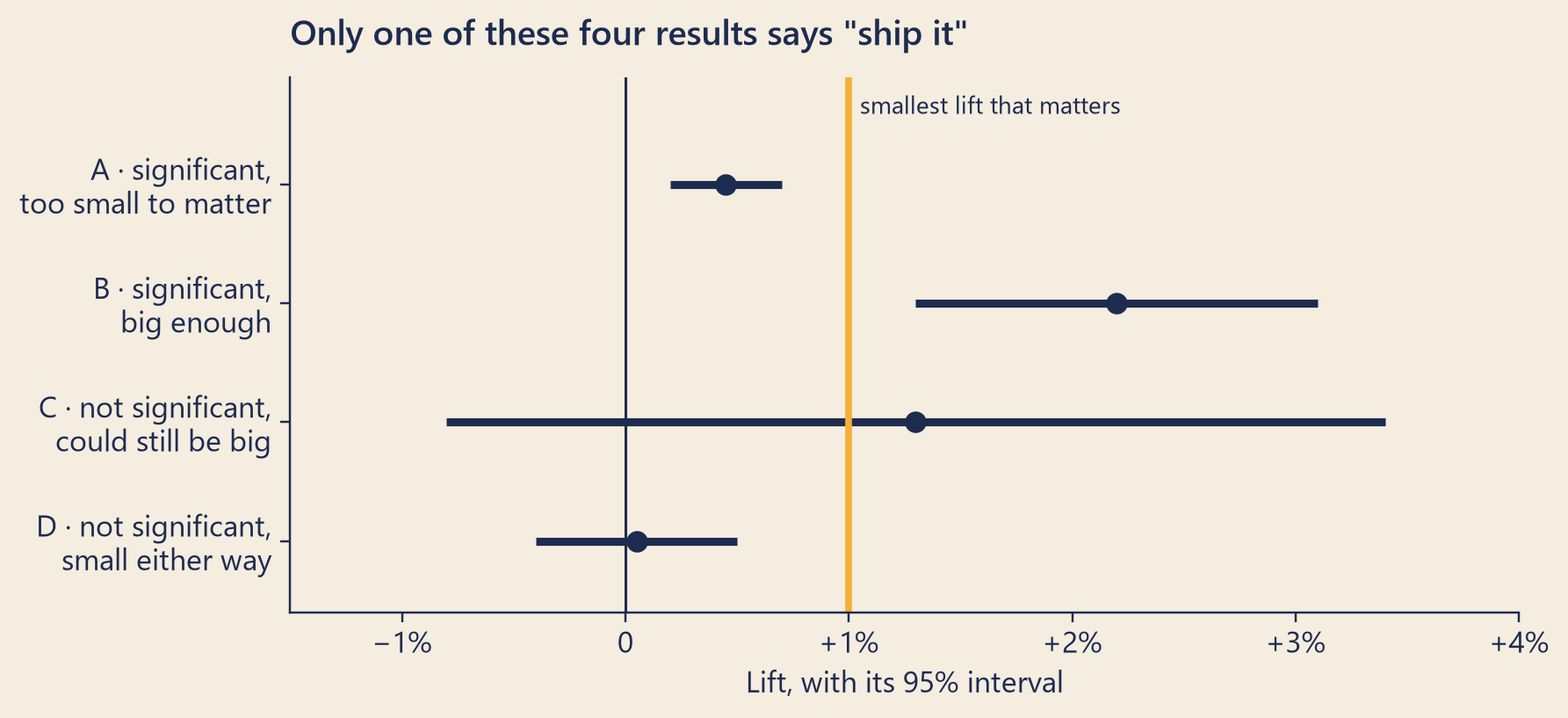
The clearest way to read a result is to put its 95% confidence interval (Chapter 17) next to two lines: zero, and the smallest effect that matters.
Show the code
examples = [("A · significant,\ntoo small to matter", 0.2, 0.7), ("B · significant,\nbig enough", 1.3, 3.1), ("C · not significant,\ncould still be big", -0.8, 3.4), ("D · not significant,\nsmall either way", -0.4, 0.5)]fig, ax = bk.figure(8, 3.6)for row, (label, lo, hi) inenumerate(reversed(examples)): ax.plot([lo, hi], [row, row], color=bk.INK, lw=3, solid_capstyle="butt") ax.plot([(lo + hi) /2], [row], "o", color=bk.INK, ms=7)ax.axvline(0, color=bk.INK, lw=1)ax.axvline(100* WORTH, color=bk.MUSTARD, lw=2.5)ax.text(100* WORTH +0.05, len(examples) -0.45, "smallest lift that matters", fontsize=9, va="bottom")ax.set_yticks(range(len(examples)), [label for label, _, _ inreversed(examples)])ax.set_ylim(-0.6, len(examples) -0.1)ax.set_xlim(-1.5, 4)ax.grid(False)ax.xaxis.set_major_formatter(plt.FuncFormatter(lambda v, _: f"{v:+.0f}%".replace("-", "−") if v else"0"))ax.set_xlabel("Lift, with its 95% interval")ax.set_title("Only one of these four results says \"ship it\"")plt.show()
Figure 3: ILLUSTRATION, not Steep data. Four possible results of a test, each shown as a 95% interval for the lift. The mustard line is the smallest lift that matters (here 1%).
A: the interval is above zero, but below 1%. The effect is probably real, and probably too small to matter.
B: the whole interval is above 1%. Real and big enough: a good reason to ship.
C: the interval is wide and crosses zero. Not significant, but the effect could still be big. The net was too small: you do not know yet.
D: the interval is narrow and sits around zero. Not significant, and any effect is too small to matter. Here, “no” is a real answer.
C and D are both “not significant”, but only D means “nothing worth having”. This is what Chapter 18 meant by “not guilty is not innocent”: before you read a “no”, you need to know how big the net was.
NoteUnder the hood
Sample size for a conversion test. Let \(p_1\) be the baseline conversion and \(p_2 = p_1(1 + \text{MDE})\). With a 50/50 split, the users needed in each group are, by the usual normal approximation,
Here \(z_q\) is the point below which a share \(q\) of the standard normal distribution lies: \(z_{0.975} = 1.96\) for alpha 0.05 (two-sided) and \(z_{0.80} = 0.84\) for power 80%. For Mia’s plan, \(p_1\) = 0.6700 and \(p_2\) = 0.6834, so \(n \approx\) 19,121.
Other splits. With a share \(s\) of users in B, the total is
which is smallest near \(s = 0.5\). When the two variances are close, a split \(s\) costs about \(1 / \big(4 s (1-s)\big)\) times the 50/50 total: about 2.8 times for 90/10.
Power and MDE. With standard error \(\text{SE} = \sqrt{p_1(1-p_1)/n_A + p_2(1-p_2)/n_B}\), the power is
where the second term (a significant result in the wrong direction) is tiny. Turned around, the MDE is about \((z_{1-\alpha/2} + z_{1-\beta}) \times \text{SE} = 2.8 \times \text{SE}\). Since \(\text{SE} \propto 1/\sqrt{n}\), the MDE falls with the square root of the sample size.
A mean, such as orders per user. For a metric with standard deviation \(\sigma\) and a change \(\delta\), \(n = 2 (z_{1-\alpha/2} + z_{1-\beta})^2 \sigma^2 / \delta^2\) per group, about \(16\,\sigma^2/\delta^2\) for alpha 0.05 and power 80%. At day 3 of the price test, \(\sigma / \mu\) = 1.27, so a 2% change needed about 63,000 users per group. That keeps the day-3 noise fixed. With more days per user, the noise shrinks relative to the mean: \(\sigma / \mu\) falls from 1.27 at day 3 to 1.10 at day 14, so the need falls as a test runs.
Duration. Mia’s table counts, for each length \(d\), the customers with a session in the \(d\) days up to 13 September and the share of them with an order in the same days. The first \(d\) with enough users is \(d\) = 9; the plan rounds up to whole weeks. Using the past to forecast the test’s traffic is itself an assumption; checkout_v2 began a week later, and Steep grows a little each week.
Counting noise versus week noise. If orders arrived independently of each other (a Poisson process), a weekly count \(A\) would have a standard deviation of \(\sqrt{A}\). The surprise of a pair of weeks would then wobble by about \(100\,(E_2/E_1)\sqrt{1/A_1 + 1/A_2}\) = 0.65 points. The summer’s pairs of weeks wobbled by 1.47: most of the noise in a weekly total is shared by the whole week. A randomised test compares groups inside the same weeks, so this shared part cancels.
The winner’s curse. Gelman and Carlin (2014) call a significant result with the wrong sign a Type S error, and the factor by which significant results overstate the truth the exaggeration ratio (a Type M error). For an estimate \(\hat\delta \sim N(\delta, \text{SE}^2)\), the exaggeration ratio is \(E\big[|\hat\delta| \,\big|\, |\hat\delta| > z_{1-\alpha/2}\,\text{SE}\big] / |\delta|\). For the day-3 look it is about 1.84; for the checkout plan at a true 1.5%, about 1.13.
Common traps
Choosing the MDE from the effect you hope for. Priya hoped for 5%. A test sized for 5% would be a small net for the smaller effects that are more common. Size the test for the smallest effect worth knowing, then decide whether you can afford it.
Stopping the moment it turns significant. The plan sets the end date. Looking early and stopping at the first good p-value breaks the promise of alpha (Chapter 21).
Partial weeks. A test that ends on a Friday gives Fridays extra weight. Run whole weeks.
“Twice the users, half the MDE.” No: twice the users shrinks the MDE by about 30%. Halving it takes four times the users.
Power after the fact. Power for the effect this same test measured adds nothing: it is the p-value in another form. Power for an effect that matters, or for one suggested by other evidence, is useful, before or after the test. That is what Chapter 18 did with a 2% drop in orders, the smallest change Dana would act on.
Reading “not significant” without the interval. Results C and D above are both “not significant”. Only the interval tells them apart.
TipAudit Instinct · How big a sample?
Auditors face Mia’s question every time they sample. Before they pick a single invoice, they decide how many to test. The auditing standard on sampling (ISA 530) lists what pushes the number up or down. Three of them map straight onto a test plan:
Tolerable misstatement: the largest error the auditor can accept in the population. It plays the part of the MDE. The smaller it is, the bigger the sample.
Expected misstatement: how much error the auditor expects to find. The closer expected error is to the most error you can accept, the bigger the sample.
The assurance wanted: how sure the auditor must be. Like a stricter alpha or a higher power, more assurance means a bigger sample.
And behind tolerable misstatement sits materiality: how big an error must be before it would change a reader’s decision. That is practical significance under another name. An auditor decides what is big enough to matter before the fieldwork, and so did Mia.
NoteInterview Corner
1. How do you calculate the sample size for an A/B test?
NoteA model answer
Pick the primary metric and measure its baseline and noise from recent data. Choose the MDE (the smallest effect worth detecting), alpha (often 0.05, two-sided), power (often 80%) and the split. Then use the standard formula: for a mean, about 16 times the variance divided by the square of the change, per group; for a proportion, its version with p(1 − p) as the variance. Turn users into days with real traffic, remembering that users accumulate slowly and conversion rises with time, and round up to whole weeks. At Steep, an MDE of 2% on a 67% conversion needed about 19,100 users per group at the two-week conversion, and two whole weeks of traffic.
2. What is the MDE, and how do you choose it?
NoteA model answer
The minimum detectable effect is the smallest true effect the test will detect with the planned power, at the planned alpha. Choose it from the business side first: the smallest effect that would change a decision (practical significance). Then check what the traffic allows. If the two do not match, make the trade-off on purpose and write it down, including the power you will have for smaller effects.
3. Traffic is too low for the MDE you want. What now?
NoteA model answer
Options, roughly in order: run longer, in whole weeks; use a 50/50 split and include more of the traffic; pick a metric closer to the change, with less noise (for example, checkout conversion rather than revenue); reduce variance with pre-test data (CUPED, Chapter 22); test a bolder change, which has a bigger effect; or accept a larger MDE and say so. What you should not do is run an underpowered test and trust a lucky significant result: the winner’s curse makes it look bigger than it is.
Reported change: −12.0% orders, the week of 7 September compared with the week before (CEO dashboard).
Explained so far: 10.1 of the 12 points (95% range 9.8 to 10.4, Chapter 17). The tracking bug, 7.0 (Chapter 15); the rainy week before, 3.4; normal growth, −0.3 (Chapter 16).
Suspects: the 5% price rise for everyone on 7 September (Priya’s price_up_5): not proved.
Ruled out: the matcha menu (Chapter 4); every stop on the data’s journey after the app (Chapters 8–14).
Open questions: About 1.9 points remain (95% range −0.7 to 4.5); the weekly numbers cannot tell them from noise (Chapter 18). What did the price test really show, and why did drinks per order step down on 7 September? Why could one look at day 3 not be trusted? (Chapter 21.)
New evidence: the power to see a real 2% drop in orders: weekly totals 33%, a look at day 3 29%, the full price test 64%. Neither yesterday’s “cannot tell” nor “it won on day 3” says much about orders; the full randomised test is the strongest evidence there is. Mia’s own test, checkout_v2, ran as planned from 21 September to 4 October; its results are opened tomorrow (Chapter 20).
Recap
Power is the chance a test catches a real effect of a given size. The MDE is the smallest effect it catches with the power you planned. Choose the MDE first, then the sample size.
Noise, effect size, alpha, power and the split set the sample size; noise and effect size count most, because users needed grow with (noise ÷ effect)². Turn users into days with real traffic, and round up to whole weeks.
Big totals are not always a big net: when whole weeks move together, comparing one week with another has little power. Randomising users over the same days cancels that shared noise.
Significant is not the same as important, and an underpowered test that wins usually wins too big. Read results as intervals next to zero and the smallest effect that matters.
English
中文
power
统计功效
minimum detectable effect (MDE)
最小可检测效应
sample size
样本量
effect size
效应量
baseline
基线
conversion
转化率
practical significance
实际显著性
statistical significance
统计显著性
underpowered
功效不足
winner’s curse
赢家诅咒
exaggeration ratio
夸大比
tolerable misstatement
可容忍错报
materiality
重要性
Further reading
Kohavi, R., Tang, D., & Xu, Y. (2020). Trustworthy Online Controlled Experiments. Cambridge University Press. DOI
Gelman, A., & Carlin, J. (2014). Beyond Power Calculations: Assessing Type S (Sign) and Type M (Magnitude) Errors. Perspectives on Psychological Science, 9(6), 641–651. DOI
Button, K. S., Ioannidis, J. P. A., Mokrysz, C., Nosek, B. A., Flint, J., Robinson, E. S. J., & Munafò, M. R. (2013). Power failure: why small sample size undermines the reliability of neuroscience. Nature Reviews Neuroscience, 14(5), 365–376. DOI
Kohavi, R., Deng, A., & Vermeer, L. (2022). A/B Testing Intuition Busters. Proceedings of the 28th ACM SIGKDD Conference on Knowledge Discovery and Data Mining, 3168–3177. DOI