On Tuesday morning, Mia copied her case board from her notebook onto a sheet of paper. She taped it to the wall by her desk.
The dashboard had shown orders down 12.0%. Most of that drop now had names. A tracking bug: 7.0 points (Chapter 15). A rainy week before the drop: 3.4 points. Normal growth, which pushes the other way: −0.3 points (Chapter 16). Together, 10.1 of the 12 points. At the bottom she wrote one more line: 1.9 points: not explained.
Theo Park, the data engineer, stopped behind her with a cup of tea. He read the sheet twice.
“One point nine,” he said. “Maybe that’s only a bad week. Orders go up and down. Nobody calls a meeting when a week is a little low.”
“Maybe,” Mia said. “Then let’s measure how surprising a week like that is.”
“Measure a surprise? With what?”
“With the summer. My recipe says how many orders a normal week should have. All summer, real weeks missed the recipe by a little, up or down. If misses like this one were common, you are right. If they were rare, something real happened.”
Theo pulled a paper napkin from his pocket. He drew a round dial with a needle and shaded a thin slice at the right end. “A surprise meter,” he said. “Most weeks, the needle stays in the big calm part. Once in a while, it swings into the thin slice. You want to know how often.”
Dana Reyes, the CEO, walked past and stopped. “Is the 1.9 real or not? The board will want a yes or a no.”
“I can tell you how surprising it is,” Mia said. “That is close to a yes or a no, but it is not the same thing. By tonight you will see the difference. First, one question: how big a change would you act on?”
Dana thought for a moment. “Two percent of orders. If the price rise or anything else cost us less than that, I would not change a thing.”
Mia wrote it down: Dana acts on 2% of orders.
ImportantThe big idea
A p-value measures how surprising your data would be if nothing had changed. It does not tell you how likely your idea is.
One number for the surprise
First, Mia wrote down exactly what she would measure. She counted completed orders: finance’s definition, with each order’s final status (see Chapter 1). These come from the orders database, so the dashboard’s bug does not touch them.
Her recipe from Chapter 16 gives the expected orders for every city and day. As in Chapter 16, she called the gap between real and expected orders the miss, now for a whole week and all four cities together. The week before the drop came in +1.5% against the recipe. The week of the drop came in −0.5%.
What matters for the case is the change between those two weeks. The recipe expected orders to change by −3.1%: the week before was rainy, and rain brings extra orders that a dry week does not repeat. Completed orders changed by −5.0%. So the change fell 1.9 points short of the recipe.
Mia called this number the surprise: the real change minus the change the recipe expected. It is roughly the second week’s miss minus the first week’s miss. So part of the 1.9 points is a week before that went unusually well, and part is a week of the drop that went a little badly.
The surprise is Mia’s test statistic: one number that sums up the data for the question she is asking. A good test statistic is far from zero when the thing you suspect is there, and close to zero when it is not.
Innocent until proven guilty
A hypothesis is a claim you can check with data. A test sets two hypotheses against each other.
The null hypothesis says nothing special happened. Here: nothing changed on 7 September. The −1.9 points are ordinary noise, the kind of surprise any pair of weeks can have.
The alternative hypothesis says something real happened. Here: something real changed orders that week, up or down, beyond the usual noise.
A hypothesis test works like a courtroom. The null hypothesis is the accused, and the accused is innocent until proven guilty. The data are the evidence. The court does not ask, “Is the accused innocent?” It asks, “Is the evidence so strong that innocence is hard to believe?”
So there are two possible verdicts. If the evidence is strong, the court says guilty: we reject the null hypothesis. If not, the court says not guilty: we fail to reject it. “Not guilty” is not the same as “innocent”. It only means the evidence was not strong enough. A careful thief with no witnesses also walks free.
Look at the picture at the top of this chapter. The teacup in the witness box is the data. The meter on the wall shows how surprising its story is. The gavel is still resting. Before the court can judge one story, it needs to know what an ordinary story sounds like.
What does an ordinary week look like?
To judge one surprise, you need to know how big ordinary surprises are: the surprises of weeks when nothing special happened. Mia called such a collection her ruler. Statisticians call it the null distribution: the spread of the test statistic when the null hypothesis is true.
The summer is the natural place to look. In Chapter 16, summer orders changed from one week to the next with a standard deviation of 2.3%. Much of that spread came from rain, which the recipe explains. So Mia worked with surprises, the part the recipe does not explain.
There is one catch, and it matters. The recipe learned from the summer weeks: it was fitted to make their misses small. A miss measured on a week the recipe learned from is called in sample. A miss measured on a week the recipe never learned from is called out of sample. The two weeks of the case came after 30 August, so their misses are out of sample. In-sample misses are a little too calm, like a student tested on the questions they practised. So the ruler for the case must be out of sample too.
A first look
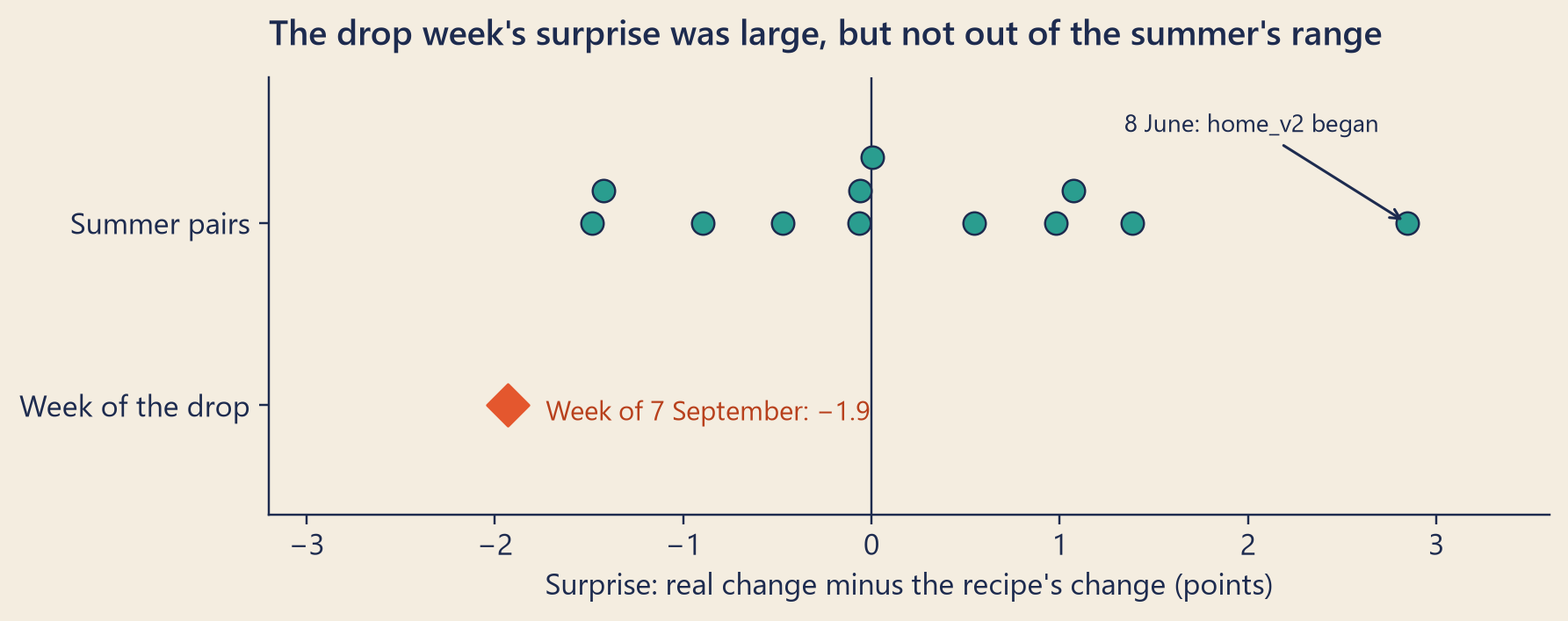
Mia first lined up the summer’s own 12 pairs of neighbouring weeks. For each pair, she computed the same number as before: the real change minus the change the recipe expected.
Show the code
fig, ax = bk.figure(8, 3.1)order = history.sort_values("surprise")ys, last_x, last_y = {}, None, Nonefor idx, row in order.iterrows(): # nudge close dots up so none hides another y =1.0if last_x isNoneor row.surprise - last_x >0.22or last_y >1.3else last_y +0.18 ys[idx], last_x, last_y = y, row.surprise, ydot_y = pd.Series(ys).reindex(history.index)ax.scatter(history.surprise, dot_y, s=70, color=bk.TEAL, edgecolor=bk.INK, lw=0.8, zorder=3)ax.scatter([observed], [0], s=120, marker="D", color=bk.TOMATO, zorder=3)ax.annotate(f"{day_month(biggest.start)}: {biggest_test} began", (biggest.surprise, dot_y[biggest.name]), xytext=(biggest.surprise -0.15, 1.5), arrowprops=dict(arrowstyle="->", color=bk.INK), ha="right", fontsize=9)ax.annotate(f"Week of {day_month(W2_START)}: {spts(observed)}", (observed, 0), xytext=(14, -3), textcoords="offset points", va="center", fontsize=10, color=bk.TOMATO_TEXT)ax.axvline(0, color=bk.INK, lw=0.8)ax.set_yticks([0, 1], ["Week of the drop", "Summer pairs"])ax.set_ylim(-0.6, 1.8)ax.set_xlim(-3.2, 3.6)ax.grid(False)ax.set_xlabel("Surprise: real change minus the recipe's change (points)")ax.set_title("The drop week's surprise was large, but not out of the summer's range")plt.show()
Figure 1: The surprise of every pair of neighbouring summer weeks (the real change minus the change the recipe expected), and of the week of the drop.
The lowest summer surprise was −1.5 points, so no summer pair fell quite as far below the recipe. But one went further from zero in the other direction: the week of 8 June beat the recipe by +2.8 points. (That was the week Steep began testing a new home screen, home_v2.)
A p-value turns this comparison into one number. It is the share of ordinary weeks that are at least as surprising as yours, if the null hypothesis is true. Here, “at least as surprising” means at least 1.9 points away from zero, in either direction. One summer pair qualifies: the week of 8 June.
When you count from a list like this, add one at the top and one at the bottom. The week you are testing is one more week that could have happened under the null hypothesis:
p = (1 + 1) / (12 + 1) = 0.154.
The +1 keeps a p-value from ever being zero. A short list can never prove that something is impossible.
This first ruler has two problems. It is in sample, so it is a little too calm. And it is short: even a week far beyond anything the summer ever saw gets p = 1/13 = 0.077. With 12 pairs, this ruler can never reach 0.05, whatever the data. Mia kept it only as a first look.
A fair ruler
So she built a better one, in two steps.
First, she made the summer misses out of sample. She refitted the recipe 13 times, each time hiding one summer week, and measured that week’s miss with the recipe that had not learned from it. The misses grew: their standard deviation went from 0.85% to 1.07%.
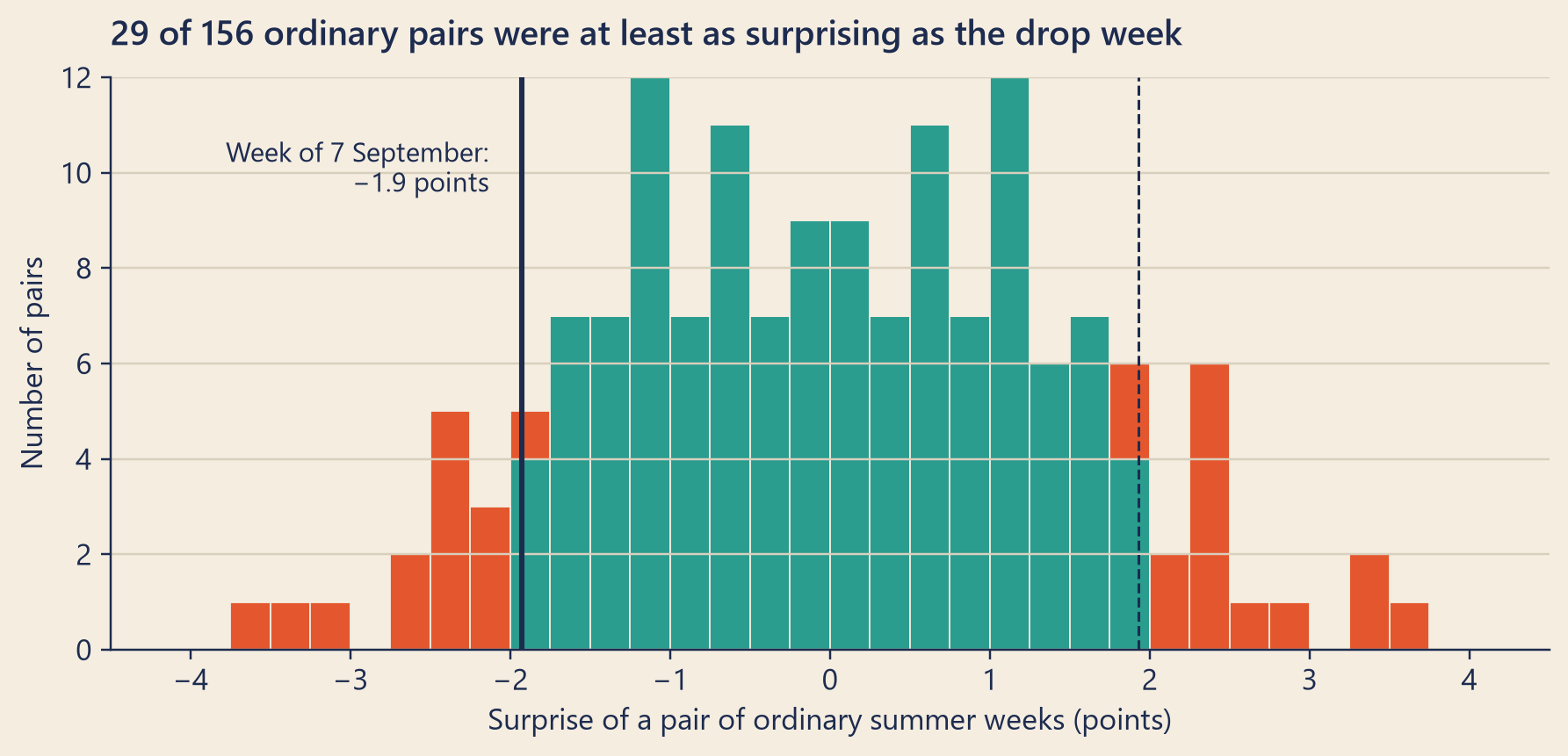
Second, she made fake pairs of weeks. Keep the real weeks’ expected orders. Swap in the misses of two summer weeks: one plays the week before, the other plays the week of the drop. Then compute the surprise, exactly as before. Thirteen summer weeks make 13 × 12 = 156 such pairs. Each pair keeps whole weeks together, as Chapter 17’s week-by-week bootstrap did, because the days of a week hang together. The pairs reuse the same 13 weeks, so they give the ruler finer marks, not more evidence. And they ignore which week came first in the summer.
Show the code
fig, ax = bk.figure(8, 3.8)bins = np.arange(-4.5, 4.51, 0.25)centres = (bins[:-1] + bins[1:]) /2in_tail = np.abs(pairs) >=abs(observed)calm, tail = np.histogram(pairs[~in_tail], bins=bins)[0], np.histogram(pairs[in_tail], bins=bins)[0]heights = calm + tailax.bar(centres, calm, width=0.25, color=bk.TEAL, edgecolor=bk.PAPER, lw=0.6)ax.bar(centres, tail, bottom=calm, width=0.25, color=bk.TOMATO, edgecolor=bk.PAPER, lw=0.6)ax.axvline(observed, color=bk.INK, lw=2)ax.axvline(-observed, color=bk.INK, lw=1, ls="--")ax.annotate(f"Week of {day_month(W2_START)}:\n{spts(observed)} points", (observed, heights.max() *0.8), xytext=(-12, 0), textcoords="offset points", ha="right", fontsize=10)ax.set_xlim(-4.5, 4.5)ax.set_xlabel("Surprise of a pair of ordinary summer weeks (points)")ax.set_ylabel("Number of pairs")ax.set_title(f"{pairs_big} of {n_pairs} ordinary pairs were at least as surprising as the drop week")plt.show()
Figure 2: The null distribution: surprises of all 156 pairs of two different summer weeks, each week’s miss measured by a recipe that did not learn from that week. Tomato parts of the bars are at least as far from zero as the week of the drop.
Of the 156 ordinary pairs, 29 were at least 1.9 points from zero, in either direction. So
p = (29 + 1) / (156 + 1) = 0.191.
That is about 1 in 5. A surprise like this is not rare.
The verdict
Before she ran either test, Mia had written two lines in her notebook: Two-sided. Call it more than noise if p < 0.05. The 0.05 is the significance level, also called alpha: how small the p-value must be before you reject the null hypothesis. You must choose it before you see the p-value. If you choose it after, you can always pick a line that gives the answer you wanted.
Alpha = 0.05 is a common convention, not a law of nature. It means you accept being fooled by noise in about 5% of ordinary weeks. When p is below alpha, people say the result is statistically significant.
Mia’s fair ruler gave p = 0.191, and her first look gave 0.154. Both are above 0.05. The test does not reject the null hypothesis: the result is not statistically significant.
Another way to see the same verdict: on the fair ruler, 95% of the ordinary surprises lie between −2.6 and +2.6 points. These are the two-sided 5% lines. A surprise outside them would have p below 0.05. The week of the drop, at −1.9, is inside.
Mia’s verdict: the weekly numbers cannot tell a 2% drop in orders (about 1.9 points of the 12) from noise.
At the end of the day, she told Dana.
“So it was noise,” Dana said.
“No,” said Mia. “It means the weekly numbers cannot tell. The court said ‘not guilty’. It did not say ‘innocent’. A real drop of 2% of orders, the size you said you would act on, could be hiding in there. A test like this would often miss it.”
“How often?”
“More often than not. Let me show you.”
Try it: the surprise meter
Move the surprise and watch the meter. The tomato part of the dial is alpha wide: if nothing changed, only that share of ordinary weeks would land there. Switch to the summer’s 12 neighbouring pairs and see how short that ruler is. (The 156 pairs here use the fair, out-of-sample misses.)
viewof meterSettings = Inputs.form({// Opens at the drop week's exact surprise (a step of 0.01 would round it and change the count).surprise: Inputs.range([-4,4], {value: meterFacts.observed,step:0.001,label:"Surprise (points)"}),ruler: Inputs.radio(newMap([["156 pairs of summer weeks","pairs"], ["12 neighbouring pairs","history"]]), {value:"pairs",label:"Compare with"}),sides: Inputs.radio(newMap([["Two-sided","two"], ["One-sided (drops only)","lower"]]), {value:"two",label:"Test"}),alpha: Inputs.radio([0.01,0.05,0.1], {value:0.05,label:"Alpha"})})
meterGauge = {const {alpha} = meterSettings;const p = meterResult.p;const C = {teal:"#2a9d8f",tomato:"#e4572e",ink:"#1d2b4f"};const cx =150, cy =140, r =108;const at = (f, rr = r) => { // f = 0 is the calm left end, f = 1 the surprising right endconst a =Math.PI* (1- f);return [cx + rr *Math.cos(a), cy - rr *Math.sin(a)]; };const arc = (f0, f1) => {const [x0, y0] =at(f0), [x1, y1] =at(f1);return`M${x0.toFixed(1)},${y0.toFixed(1)} A${r},${r} 0 0 1 ${x1.toFixed(1)},${y1.toFixed(1)}`; };const [nx, ny] =at(Math.min(1,Math.max(0,1- p)), r -22);return htl.svg`<svg viewBox="0 0 300 175" width="300" style="max-width:100%;height:auto;display:block;margin:0 auto" role="img" aria-label="Surprise meter: the needle sits at ${(100* (1- p)).toFixed(1)} percent of the dial"> <path d="${arc(0,1- alpha)}" stroke="${C.teal}" stroke-width="24" fill="none"/> <path d="${arc(1- alpha,1)}" stroke="${C.tomato}" stroke-width="24" fill="none"/> <line x1="${cx}" y1="${cy}" x2="${nx.toFixed(1)}" y2="${ny.toFixed(1)}" stroke="${C.ink}" stroke-width="5" stroke-linecap="round"/> <circle cx="${cx}" cy="${cy}" r="8" fill="${C.ink}"/> <text x="${cx - r}" y="${cy +28}" text-anchor="middle" font-size="13" fill="${C.ink}">calm</text> <text x="${cx + r -10}" y="${cy +28}" text-anchor="middle" font-size="13" fill="${C.ink}">surprising</text> </svg>`;}
Show the code
meterReadout = {const {ruler, alpha} = meterSettings;const {p, hits, total} = meterResult;const n =1/ p;const oneIn = n <10? n.toFixed(1) :Math.round(n).toLocaleString("en-US");const what = ruler ==="history"?"neighbouring summer pairs":"pairs of summer weeks";const floor =html`<p>With ${total}${what}, this ruler can never show p below 1/${total +1} = ${(1/ (total +1)).toFixed(3)}.</p>`;const verdict = p < alpha?`p is below alpha (${alpha}): statistically significant. A week like this would be rare if nothing had changed.`:`p is not below alpha (${alpha}): not statistically significant. This does not prove that nothing changed.`;returnhtml`<p>${hits} of the ${total}${what} were at least this surprising.</p> <p>p = (${hits} + 1) / (${total} + 1) = <strong>${p.toFixed(3)}</strong>, about 1 in ${oneIn}.</p>${floor} <p><strong>${verdict}</strong></p>`;}
Try −1.0, then −3.0, and switch between the two rulers. The one-sided test counts only drops, so a big rise never looks surprising to it.
Two ways to be wrong
A court can make two kinds of mistakes, and so can a test.
Nothing really changed
Something really changed
Test says “significant”
Type I error: a false alarm. An innocent person goes to jail.
Correct: a real change found.
Test says “not significant”
Correct: noise called noise.
Type II error: a miss. A guilty person walks free.
When nothing changed, the chance of a Type I error is alpha. You chose it. With alpha = 0.05, about 1 ordinary week in 20 sets off the alarm.
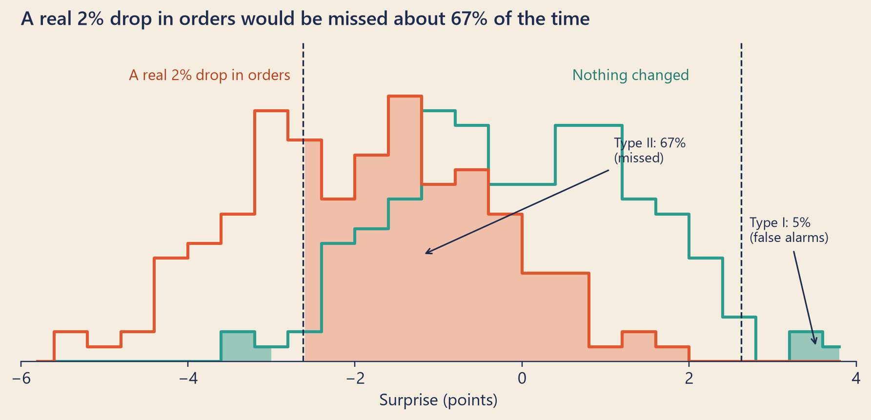
The chance of a Type II error depends on how big the real change is, and on how noisy the data are. To measure it, Mia needed a size that matters, chosen from outside the test. Dana had given her one that morning: a drop of 2% in orders is the smallest change Dana says she would act on. (Chapter 19 calls this practical significance: a change big enough to matter.) In points of the 12, it is a little less than 2, because the week of the drop was 5.0% smaller than the week before: 2 × 0.950 ≈ 1.9 points. Mia moved every one of the 156 ordinary surprises down by that much. Then she counted how many still stayed between the two-sided 5% lines, at ±2.6 points.
Show the code
fig, ax = bk.figure(8, 3.8)bins = np.arange(-6, 4.01, 0.4)centres = (bins[:-1] + bins[1:]) /2h0 = np.histogram(pairs, bins=bins)[0]h1 = np.histogram(pairs - drop_pts, bins=bins)[0]outside = np.abs(centres) >= critax.fill_between(centres, h0, where=outside, step="mid", color=bk.TEAL, alpha=0.45, lw=0)ax.fill_between(centres, h1, where=~outside, step="mid", color=bk.TOMATO, alpha=0.3, lw=0)ax.step(centres, h0, where="mid", color=bk.TEAL, lw=2)ax.step(centres, h1, where="mid", color=bk.TOMATO, lw=2)for x in (-crit, crit): ax.axvline(x, color=bk.INK, ls="--", lw=1.1)top =max(h0.max(), h1.max())ax.text(0.6, top *1.06, "Nothing changed", ha="left", color=bk.TEAL_TEXT, fontsize=10)ax.text(-crit -0.15, top *1.06, f"A real {bk.fmt_pct(REAL_CUT, 0)} drop in orders", ha="right", color=bk.TOMATO_TEXT, fontsize=10)ax.annotate(f"Type II: {bk.fmt_pct(1- power_drop, 0)}\n(missed)", (-1.2, top *0.4), xytext=(1.1, top *0.75), arrowprops=dict(arrowstyle="->", color=bk.INK), fontsize=9)ax.annotate(f"Type I: {bk.fmt_pct(ALPHA, 0)}\n(false alarms)", (crit +0.9, top *0.05), xytext=(crit +0.1, top *0.45), arrowprops=dict(arrowstyle="->", color=bk.INK), fontsize=9)ax.set_ylim(0, top *1.2)ax.set_xlim(-6, 4)ax.set_yticks([])ax.grid(False)ax.spines["left"].set_visible(False)ax.set_xlabel("Surprise (points)")ax.set_title(f"A real {bk.fmt_pct(REAL_CUT, 0)} drop in orders would be missed about "f"{bk.fmt_pct(1- power_drop, 0)} of the time")plt.show()
Figure 3: Two worlds, one rule. Teal: the 156 ordinary surprises, if nothing changed. Tomato: the same surprises if something real cost 2% of the week’s orders (1.9 points). The dashed lines are the two-sided 5% lines.
About 67% did. So if something real cost 2% of the orders, this test would miss it more often than it would catch it. The other 33% is the test’s power for a 2% drop: the chance it catches a real change of that size. Chapter 19 is about power.
This is why Mia would not say “it was noise”. With so little power, “not significant” was the likely result whether or not something real happened. A test that would usually say “not significant” anyway does not prove that nothing happened. In short: absence of evidence is not evidence of absence.
The two errors pull against each other. A stricter alpha, such as 0.01, gives fewer false alarms but more misses. Only better evidence, more data or less noise, reduces both.
One side or two?
Mia’s p-values counted surprises in both directions: pairs at least 1.9 points below the recipe, and pairs at least 1.9 points above it. That is a two-sided test. A one-sided test counts only one direction, here only drops. Its p-value is about half.
Here, a one-sided test on Mia’s fair ruler gives p = 0.096: still above 0.05.
A one-sided test is fair only when two things are true. You chose the direction before you saw the data. And a surprise in the other direction would not change what you do. Mia had seen the direction before she started: the whole case is about a drop. Choosing a one-sided test now would halve the p-value for free. That is why her notebook said “two-sided” first.
How big could the last 1.9 points be?
Chapter 17 gave a range for every number on the case board except the last 1.9 points. Mia could give one now, with the same ruler. Noise can move a surprise about 2.6 points either way, so the true unexplained drop is somewhere from −0.7 to 4.5 points.
The range includes 0, so the weekly numbers cannot rule out “nothing else happened”. It also includes 2 and 3, so they cannot rule out a real cost of a few points either.
What a p-value is not
In 2016, the American Statistical Association published a short statement on p-values, because so many people misread them (Wasserstein and Lazar, 2016). Here is what its principles mean for the week of the drop.
p = 0.191 does not mean “a 19.1% chance that it was noise”, or “an 80.9% chance that something real happened”. It means: if it was noise, a pair of weeks this surprising would turn up about 19.1% of the time. These are different questions. Compare: “If someone plays professional basketball, how likely is that person to be tall?” (very likely) and “If someone is tall, how likely is that person to play professional basketball?” (very unlikely).
p above 0.05 does not mean nothing happened. It means this evidence is not strong enough to say so.
p does not say how big the real change is. The 1.9 points is the size; the range above says how sure we are about it.
A p-value is only as good as its picture of “ordinary”. Mia’s rulers gave 0.154 and 0.191. A careless ruler built from single days would have given 0.013 and an overconfident “significant” (Under the hood shows why). That is why Mia wrote down every ruler she tried: the ASA statement asks for full reporting.
NoteUnder the hood
The test statistic. Let \(A_1, A_2\) be real orders in the week before and the week of the drop, and \(E_1, E_2\) the recipe’s expected orders. The weekly miss is \(r_k = A_k / E_k - 1\), and the surprise, in points, is
For the week of the drop, \(r_1\) = +0.0148, \(r_2\) = −0.0054 and \(S\) = −1.929, exactly minus the case board’s open points. Over the 13 summer weeks, the misses \(r_k\) have a standard deviation of 0.85% in sample, and 1.07% when each week is left out of the fit that judges it (leave-one-out, a form of cross-validation). Both \(r_1\) and \(r_2\) are out of sample, so the second is the fair comparison.
The rulers. Ruler 2 keeps \(E_1, E_2\) and replaces \((r_1, r_2)\) by the out-of-sample misses of two different summer weeks \((r_a, r_b)\), for all 13 × 12 ordered pairs. This treats the summer weeks as exchangeable under the null: any week’s miss could have landed on any week. With \(N\) ordinary surprises \(S^*_j\), the two-sided p-value is
The \(+1\) counts the observed pair itself, so \(p\) is never zero (Phipson and Smyth, 2010).
Why does the short ruler give 0.154 while all 156 in-sample pairs give 0.076? The short ruler’s one big surprise, 8 June, came from two unusual weeks side by side: a low first week of June, then a high week. On the short ruler, that is 1 of 12 pairs. Among all 156 pairs, those two weeks meet in only 2. The long ruler judges each week’s miss, not the luck of which weeks happened to be neighbours.
How “ordinary” was built
Two-sided p
One-sided p
The summer’s 12 neighbouring pairs, counted (in sample)
0.154
0.077
A t curve with 11 degrees of freedom and their spread (sd 1.25)
0.151
0.075
All 156 pairs, in-sample misses: too calm
0.076
0.038
All 156 pairs, out-of-sample misses (sd 1.47): the main ruler
0.191
0.096
All 210 pairs of 15 weeks (the summer, plus the two weeks of the case), exact
0.100
0.048
Weeks built from single summer days (sd 0.78): far too narrow
0.013
0.006
Why the last ruler is wrong. It draws 14 summer days at random, 100,000 times, as if each day’s miss were independent of the next. Its spread, 0.78 points, is far narrower than what real summer weeks did (1.25 to 1.47). The main reason is causes that last a whole week, such as a holiday, a local event or one of Steep’s own tests: they move all seven days together, and drawing single days spreads them thin. The link between neighbouring days is small (a correlation of 0.14, as Chapter 17 found); on its own, it would widen a 7-day sum only by a factor of about 1.12 (from 0.78 to 0.88). Build the null at the level of the test statistic: weeks, not days. And always check a simulated null against real history.
The range. If the true unexplained drop is \(\delta\) points, then \(S \approx -\delta + \text{noise}\). Taking the noise from the main ruler, with 2.5% and 97.5% points \(q_{lo}\) and \(q_{hi}\), gives the 95% range \([-S - q_{hi},\; -S - q_{lo}]\) = −0.7 to 4.5. These are the \(\delta\) values for which the two-sided test would not reject.
Errors and power.\(\alpha = P(\text{reject } H_0 \mid H_0 \text{ true})\) and \(\beta = P(\text{fail to reject } H_0 \mid H_1 \text{ true})\). Power is \(1 - \beta\). For a true drop of \(\delta\) points and a bell-shaped null with standard deviation \(\sigma\), power \(\approx \Phi(\delta / \sigma - z_{1-\alpha/2})\), where \(\Phi\) is the standard normal distribution function. A loss of 2% of the week’s orders gives \(\delta = 2 A_2 / A_1\) = 1.90 points. With \(\sigma\) = 1.47, that is 0.25; counting the shifted pairs gave 0.33. The 156 pairs are not quite bell-shaped, so the two differ: with so few weeks, both numbers are rough. The size 2% was chosen from the question (what would close the case), not from this test’s own estimate: power computed for the effect a test measured adds nothing (Chapter 19).
Naming a suspect
The test could not say whether something real happened. But a court does not stop at one witness. Mia had other evidence, and it did not come from weekly totals.
First, in every city, the change from the week before fell short of the recipe, even in the two dry cities (Chapter 16). The cities share one week, so this supports the case but does not prove it. Second, something did change that week. Mia listed what changed. iOS 3.2.0 came out, but its bug only hid orders from the dashboard (Chapter 15); her counts are completed orders from the orders database, not app events, so the bug is not in them. The weather was already in the recipe. That left one more change.
“Prices,” Theo said. “Priya’s price test, back in August. Half the users saw prices 5% higher. It was called a win after three days, and the new prices went live for everyone on 7 September.”
Mia checked the order lines. On 6 September, a Classic Milk Tea cost $4.50. On 7 September, it cost $4.75. Every drink on the menu went up by between 4.8% and 5.6% (prices are rounded to 5 cents).
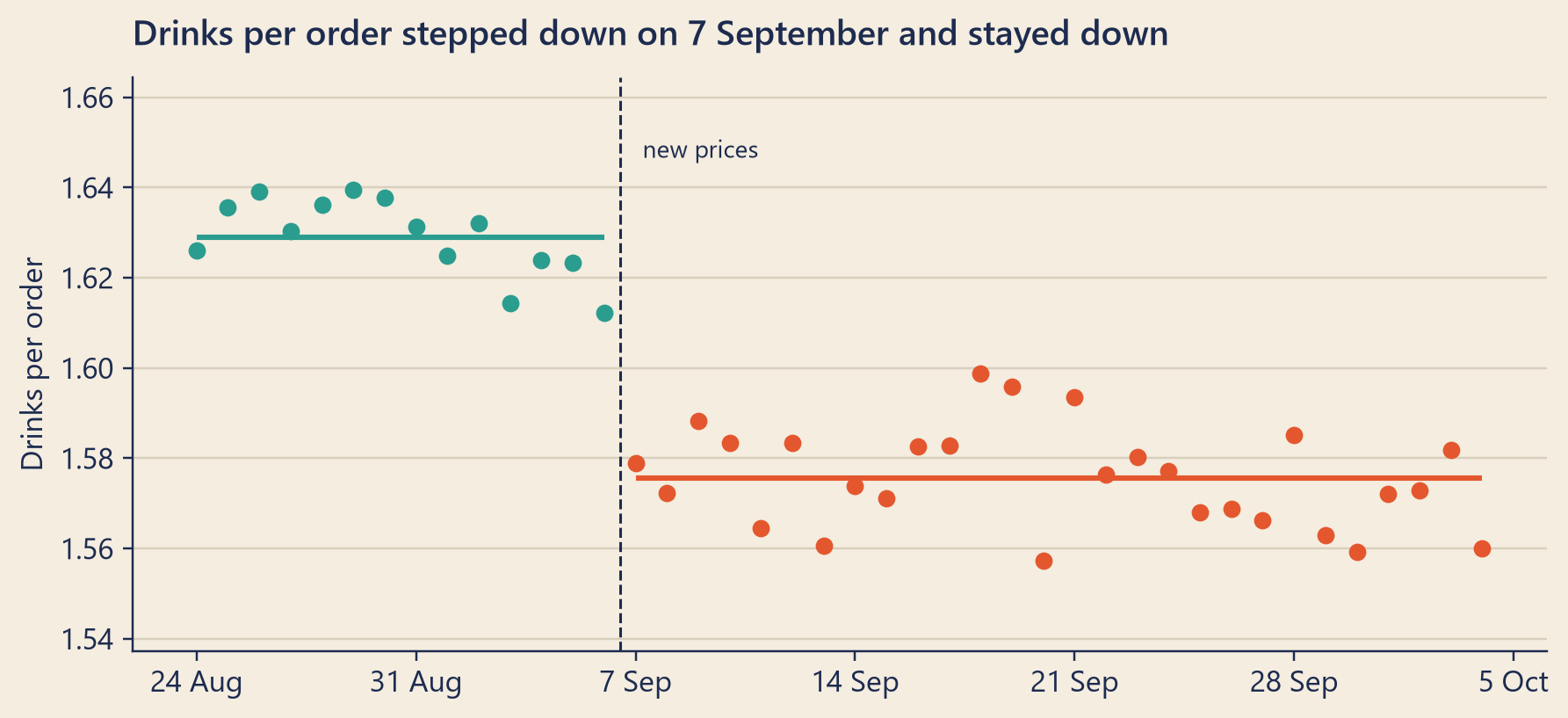
A higher price is a natural suspect for fewer orders. It also fits an old clue. In Chapter 2, Mia saw that drinks per order fell 3.0% in the week of the drop, while the money per order rose. She wrote it down as a question. Now she looked at it day by day.
Show the code
fig, ax = bk.figure(8, 3.6)is_after = drinks.day >= PRICE_DAYax.scatter(drinks.day[~is_after], drinks.drinks_per_order[~is_after], color=bk.TEAL, s=30, zorder=3)ax.scatter(drinks.day[is_after], drinks.drinks_per_order[is_after], color=bk.TOMATO, s=30, zorder=3)ax.hlines(dpo_before, DRINKS_FROM, PRICE_DAY - pd.Timedelta(days=1), color=bk.TEAL, lw=2)ax.hlines(dpo_after, PRICE_DAY, DRINKS_TO, color=bk.TOMATO, lw=2)ax.axvline(PRICE_DAY - pd.Timedelta(hours=12), color=bk.INK, ls="--", lw=1)top = drinks.drinks_per_order.max()ax.text(PRICE_DAY, top +0.006, " new prices", fontsize=9, va="bottom")ax.set_ylim(drinks.drinks_per_order.min() -0.02, top +0.025)ax.xaxis.set_major_locator(mdates.WeekdayLocator(byweekday=mdates.MO))ax.xaxis.set_major_formatter(plt.FuncFormatter(lambda v, _: f"{mdates.num2date(v):%d %b}".lstrip("0")))ax.set_ylabel("Drinks per order")ax.set_title(f"Drinks per order stepped down on {day_month(PRICE_DAY)} and stayed down")plt.show()
Figure 4: Drinks per order for regular customers (not corporate accounts), each day from the end of the price test to last Sunday. Lines show the average before and after 7 September.
Drinks per order did not drift down. For regular customers, they stepped down on 7 September and stayed down: from 1.63 on average in the two weeks before, to 1.58 in the four weeks after (−3.3%). Every day after the price change was lower than every day before it.
Mia wrote in her notebook: Suspect: the 5% price rise for everyone, 7 Sep. Not proved.
Why not proved? Because “something changed on 7 September” and “prices rose on 7 September” fit together, but fitting is not proof. Other things could have changed that day, too: a rival’s special offer, the start of the school year, a change that nobody wrote down. As the Prologue warned, a story that fits is not the same as a story that is true.
And the weekly totals cannot settle it. A change of about 2% is too small for them to see reliably: the power above was only 33%. Chapter 19 explains why, and why the same was true of a test that looked after three days. To prove that the price rise cost orders, Mia needs a comparison in which the price is the only difference. Steep has one: price_up_5 itself, where users were split at random. Chapter 21 re-runs that test with all of its days, and explains the drinks per order.
Common traps
“Not significant, so nothing happened.” No. “Not guilty” is not “innocent”. A test with low power usually says “not significant” even when something real happened. Look at the power and the range before you say “nothing”.
“p = 0.191, so there is an 81% chance the change is real.” No. The p-value assumes the null hypothesis is true and asks how surprising the data are. It cannot tell you how likely the null hypothesis is.
Choosing after you look. Picking the ruler, the side (one or two) or alpha after seeing the result can turn “not significant” into “significant”. Here, a one-sided test on the too-calm in-sample ruler (Under the hood) gives p = 0.038: chosen after seeing the drop, it would have flipped Mia’s verdict. Write your choices down first, and report every ruler you tried.
A null that is too narrow. Building “ordinary” from small pieces that are not independent, such as single days, makes ordinary look calmer than it is. Real surprises then look rare. Build the null at the level of your test statistic, and check it against history.
Significant means important. A tiny change can be significant with enough data. Chapter 19 separates “real” from “big enough to matter”.
TipAudit Instinct · Negative and positive assurance
Auditors choose their words with care. After an audit, they give positive assurance: “In our opinion, the financial statements are presented fairly.” They gathered enough evidence to say so.
After a review, which is a smaller job, they give negative assurance: “Nothing has come to our attention that causes us to believe the statements are not presented fairly.” This does not say the statements are fair. It says the review found no problem. A small review can miss things.
A hypothesis test speaks the same careful language. Mia’s weekly test gave negative assurance about noise: nothing in the weekly totals proves that something changed. That is not the same as “nothing changed”, and her report to Dana said so. And like a reviewer with more questions, she knew where to look for stronger evidence: a randomised test.
NoteInterview Corner
1. What is a p-value?
NoteA model answer
Assume the null hypothesis is true: nothing changed. The p-value is the probability of getting a test statistic at least as extreme as the one you observed. It measures how surprising the data are under that assumption. It is not the probability that the null hypothesis is true, and it does not measure the size or importance of an effect. At Steep, the week of the drop fell 1.9 points below the recipe (the expectation model); against every pair of summer weeks, the two-sided p was 0.191.
2. What is the difference between a Type I and a Type II error?
NoteA model answer
A Type I error is a false positive: you reject the null hypothesis when nothing changed. Its rate is alpha, which you choose. A Type II error is a false negative: you miss a real effect. Its rate, beta, depends on the effect size, the noise and the sample size; power is 1 − beta. For a fixed amount of data, lowering alpha raises beta. More data, or less noise, lowers beta at the same alpha, or lets you lower both.
3. Your test is not significant. What can you conclude?
NoteA model answer
Only that the data did not give strong evidence against the null hypothesis. It is not proof of no effect. Check two things. First, the range for the effect: if it is narrow and close to zero, any effect is probably too small to matter; if it is wide, the data cannot tell. Second, the power for an effect size that matters. At Steep, the weekly test had about 33% power for a real 2% drop in orders, and the range for the open points ran from −0.7 to 4.5, so “not significant” meant “cannot tell”, not “nothing happened”.
Reported change: −12.0% orders, the week of 7 September compared with the week before (CEO dashboard).
Explained so far: 10.1 of the 12 points (95% range 9.8 to 10.4, Chapter 17). The tracking bug, 7.0 (Chapter 15); the rainy week before, 3.4; normal growth, −0.3 (Chapter 16).
Suspects: the 5% price rise for everyone on 7 September (Priya’s price_up_5, called a win after three days): not proved.
Ruled out: the matcha menu (Chapter 4); every stop on the data’s journey after the app (Chapters 8–14).
Open questions: About 1.9 points remain (95% range −0.7 to 4.5). The weekly numbers cannot tell a 2% drop in orders (about 1.9 points of the 12) from noise (p = 0.191, two-sided, this chapter). Why can weekly totals, or a test read after three days, not see a 2% change? (Chapter 19.) What did the price test really show, and why did drinks per order step down on 7 September? (Chapter 21.)
New evidence: drinks per order stepped down on the day the new prices started, and stayed down.
Recap
A hypothesis test asks: if nothing had changed, how surprising would these data be? The p-value is that surprise, as a probability.
The answer depends on your picture of “ordinary”, the null distribution. Build it at the level of your test statistic, choose alpha and the side before you look, and report every ruler you tried.
“Not significant” is not “nothing happened”: a test with low power usually misses real changes. Report the power and the range, not only the verdict.
English
中文
hypothesis
假设
null hypothesis
原假设 / 零假设
alternative hypothesis
备择假设
test statistic
检验统计量
miss (residual)
残差
null distribution
零分布
p-value
p 值
significance level (alpha)
显著性水平
statistically significant
统计显著
Type I error
第一类错误
Type II error
第二类错误
power
统计功效
one-sided / two-sided test
单侧 / 双侧检验
absence of evidence
缺乏证据(不等于没有)
negative assurance
消极保证
Further reading
Wasserstein, R. L., & Lazar, N. A. (2016). The ASA Statement on p-Values: Context, Process, and Purpose. The American Statistician, 70(2), 129–133. DOI
Greenland, S., Senn, S. J., Rothman, K. J., Carlin, J. B., Poole, C., Goodman, S. N., & Altman, D. G. (2016). Statistical tests, P values, confidence intervals, and power: a guide to misinterpretations. European Journal of Epidemiology, 31(4), 337–350. DOI
Phipson, B., & Smyth, G. K. (2010). Permutation P-values Should Never Be Zero: Calculating Exact P-values When Permutations Are Randomly Drawn. Statistical Applications in Genetics and Molecular Biology, 9(1). DOI