On Monday morning, Dana came to Mia’s desk with Friday’s page in her hand. She had underlined one number twice.
“You told me 3.4 points for the rain,” she said. “How sure are you? The board will ask. Someone always asks.”
“Fairly sure that it is more than three,” said Mia. “Not sure of the decimal.”
“I cannot say ‘not sure of the decimal’ to a board.”
“Then I will give you a range. A low number and a high number, and how often a range like that is right.”
Theo rolled his chair over. “And then ask her how sure she is about the range.”
Dana ignored him. “One sentence for each number, please. Something I can say out loud.” She left the page on the desk.
Mia looked at it. Every number on it came from data, and every one of them would have come out a little different with different data. The 3.4 points came from one summer: thirteen weeks of weather and orders. Another summer, with rain on different days, would have taught the recipe a slightly different rain factor. The question was not whether the number would move, but how far.
ImportantThe big idea
Every estimate comes with a range. Report the range, and know what it means.
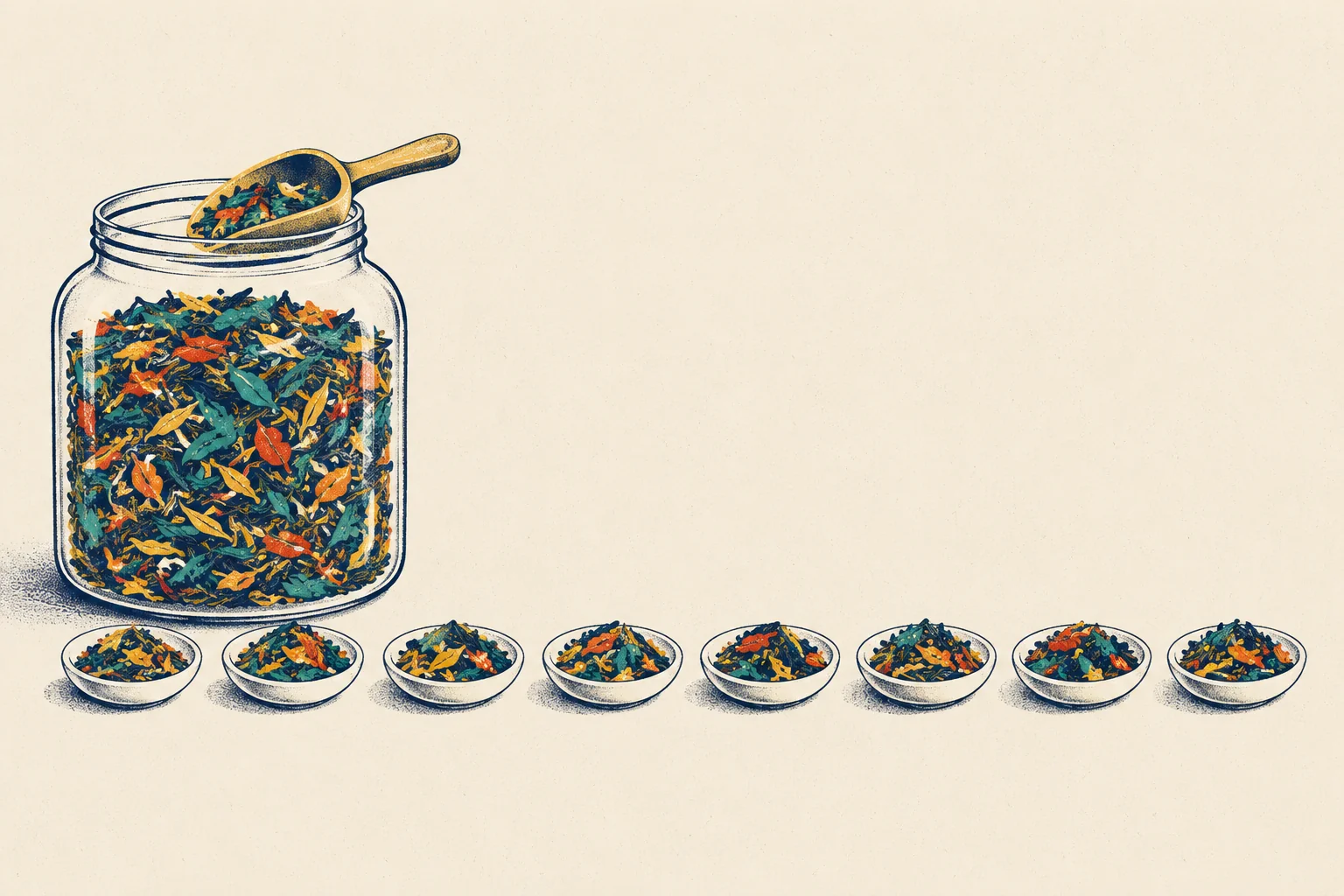
Look at the eight dishes in the picture. Each one is a scoop from the same jar, yet no two mixes are quite the same. If you judged the jar by one dish, you would be a little wrong, and you would not know by how much, unless you looked at how different the dishes are from each other. That difference is what this chapter measures.
Two kinds of spread
Chapter 16 used the standard deviation (SD) to say how spread out values are. This chapter needs a second kind of spread, and the two are easy to mix up.
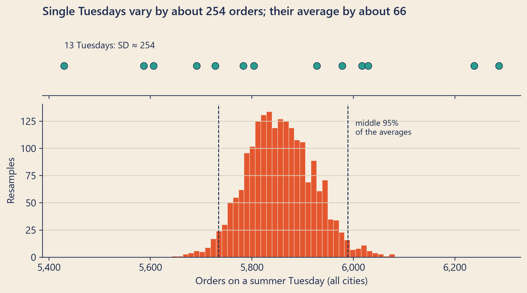
Take the summer’s Tuesdays. Steep had thirteen of them, with 5,854 orders on average (all four cities together). A typical Tuesday sat about 254 orders away from that average: that is their standard deviation, the typical distance from the average. (Two Tuesdays picked at random differ by more, about 1.4 SD.) The SD describes single Tuesdays.
But Mia’s recipe does not use single Tuesdays. It uses all thirteen together, like an average. So the useful question is a different one. If Steep could live the summer again, with new luck, how much would the average of thirteen Tuesdays move?
The answer has its own name: the standard error (SE). It is the standard deviation of an estimate, such as an average, across all the samples you might have drawn. For an average of independent values, there is a simple rule. (Independent means that knowing one value tells you nothing about the others.) Divide the SD by the square root of the number of values.
SE = 254.2 ÷ √13 ≈ 70.5 orders.
In the picture’s terms: the SD is about the leaves, how different one leaf is from another. The SE is about the dishes, how different one scoop’s mix is from another’s. A bigger scoop holds more leaves, so its mix is closer to the jar’s, and the dishes differ less. The SE shrinks as the sample grows; the SD does not.
The bootstrap: summers you did not have
The rule “SD ÷ √n” works for an average. Mia’s rain points are not an average. They come out of a recipe with twelve numbers, fitted on 364 city-days, then applied to two other weeks. There is no simple rule for that.
She cannot live the summer again either. But she can do the next best thing. The idea is called the bootstrap, and it fits in one sentence: treat your sample as if it were the population, and draw new samples from it.
Here is how it works on the Tuesdays.
Put the thirteen Tuesdays in a hat.
Draw one, write it down, and put it back. Do this thirteen times. Some Tuesdays get picked twice, some not at all. In one such draw, three Tuesdays were picked more than once and four were not picked.
Average the thirteen you drew. That is one resample: a new sample made from the old one.
Repeat 2,000 times.
Each resample is a summer that could have happened, built from pieces of the summer that did. The spread of their averages shows how much the average moves from one possible summer to another.
Show the code
bk.setup()fig, (top, bottom) = plt.subplots(2, 1, figsize=(8, 4.4), sharex=True, layout="constrained", gridspec_kw={"height_ratios": [1, 2.2]})top.scatter(tuesdays, np.zeros(n_tue), s=60, color=bk.TEAL, edgecolor=bk.INK, lw=0.6, zorder=3)top.set_yticks([])top.grid(False)top.spines["left"].set_visible(False)top.set_title(f"Single Tuesdays vary by about {tue_sd:,.0f} orders; their average by about {boot_tue_se:,.0f}")top.text(tuesdays.min(), 0.35, f"{n_tue} Tuesdays: SD ≈ "+ bk.fmt_int(tue_sd), fontsize=10)top.set_ylim(-0.6, 0.8)bottom.hist(boot_tue, bins=40, color=bk.TOMATO, edgecolor=bk.PAPER, lw=0.4)for edge in (tue_lo, tue_hi): bottom.axvline(edge, color=bk.INK, ls="--", lw=1)bottom.text(tue_hi +15, bottom.get_ylim()[1] *0.8, "middle 95%\nof the averages", fontsize=9)bottom.set_ylabel("Resamples")bottom.set_xlabel("Orders on a summer Tuesday (all cities)")bottom.xaxis.set_major_formatter(mticker.FuncFormatter(lambda v, _: f"{v:,.0f}"))plt.show()
Figure 1: Top: the summer’s Tuesdays, all cities together. Bottom: the averages of the bootstrap resamples of those Tuesdays. Same axis, very different spreads.
The 2,000 averages have a standard deviation of 66 orders. That is the bootstrap standard error, close to the rule’s 70.5. (With only thirteen values the bootstrap runs a little low; “Under the hood” says why.)
A range built by a method that aims to catch the true value 95 times in 100 is called a 95% confidence interval. (The next sections say exactly what that means.) The middle 95% of the averages runs from 5,734 to 5,989. That is a bootstrap range for the average summer Tuesday, not for any single Tuesday: single Tuesdays ran from 5,430 to 6,287. With only thirteen values it is a little too narrow (“Under the hood” says by how much). A quick 95% range from the formula is the average ± about 2 SE; with 13 values, use 2.18 instead of 2. That gives 5,701 to 6,008.
The bootstrap was introduced by the statistician Bradley Efron in 1979. Its name comes from an old saying about lifting yourself up by your own bootstraps, the loops on the back of a boot: an impossible trick. Here, the data seem to lift themselves: they measure their own uncertainty, with no new data and no formula.
A range for the rain
Now Mia did the same with the whole recipe. One resample worked like this:
Draw 91 days from the 91 summer days, with replacement. Each day comes with all four cities.
Fit the recipe again on that resampled summer.
Ask the new recipe how many points of the fall from W1 to W2 (the week before the drop, and the week of the drop) the rain explains.
She did this 2,000 times.
Show the code
fig, axes = plt.subplots(2, 1, figsize=(8, 4.6), sharex=True, layout="constrained")for ax, frame, label, (lo, hi) in [(axes[0], boot_days, "Resampling single days", rain_day), (axes[1], boot_weeks, "Resampling whole weeks", rain_week)]: ax.hist(frame.rain_pts, bins=np.arange(2.7, 4.1, 0.025), color=bk.MUTED, edgecolor=bk.PAPER, lw=0.3)for edge in (lo, hi): ax.axvline(edge, color=bk.INK, ls="--", lw=1.1) ax.axvline(weather_pts, color=bk.TOMATO, lw=2) ax.text(0.995, 0.85, label +":\n"+ span(lo, hi) +" points", transform=ax.transAxes, fontsize=10, ha="right") ax.set_ylabel("Resamples")axes[0].set_title(f"Resampled summers put the rain at about {span(rain_lo, rain_hi)} points")axes[1].set_xlabel("Points of the fall explained by rain")plt.show()
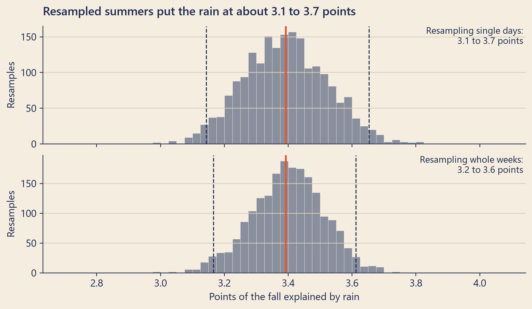
Figure 2: The rain’s share of the fall in each bootstrap resample of the summer. Top: resampling single days. Bottom: resampling whole weeks. Dashed lines: the middle 95%. Tomato line: the recipe fitted on the real summer.
The middle 95% runs from 3.1 to 3.7 points. The bootstrap standard error is 0.13 points. In the same resamples, the rain factor itself ran from × 1.104 to × 1.122.
When neighbouring days are linked
Resampling single days quietly assumes that days are independent: that knowing one day’s luck tells you nothing about the next day’s. If days are linked, that is wrong. Rain comes in wet spells. A busy day can leave the stores short of staff the next morning. Anything the recipe does not know about, and that lasts a few days, links neighbouring days.
Linked days carry less information than the same number of separate days. Resampling single days pulls the links apart, so the bootstrap thinks it has 91 separate pieces of evidence when it really has fewer. The range comes out too narrow.
The safer way is a block bootstrap: resample whole blocks of neighbouring days, and keep each block together. Weeks are natural blocks here, because every week holds each weekday once. The bottom half of the chart resamples the thirteen summer weeks, and gives 3.2 to 3.6 points.
For the rain, the two agree. The misses of neighbouring days are only weakly linked. Their correlation, a number from −1 to 1 that says how closely two things move together (0 means not at all), is 0.14. Here the “safer” week version came out a little narrower. That does not mean the days are fine: with only thirteen blocks, the block bootstrap is unstable itself. That is why Mia takes the wider of the two ranges. Mia’s range for the rain is 3.1 to 3.7 points.
For growth they do not agree: whole weeks give a much wider range, 0.13 to 0.43% per week against 0.19 to 0.38% from single days. The recipe learns growth by comparing early and late weeks. One lucky week can tilt it. Mia uses the wider range for growth too.
{// The last resample, as a calendar: one column per summer week, one row per weekday.const counts = bootRun.lastCounts;const days = ["Mon","Tue","Wed","Thu","Fri","Sat","Sun"];const shade = (k) => k ===0?"transparent": k ===1?"#a8d5cf": k ===2? C17.teal: C17.ink;const cell = (k) => {const td =document.createElement("td"); td.textContent= k ===0?"": k; td.style.cssText=`width:1.25rem;height:1.05rem;text-align:center;font-size:0.62rem;border-radius:2px; border:1px solid rgba(29,43,79,0.25);background:${shade(k)};color:${k >=2?"#fffdf8": C17.ink}`;return td; };const table =document.createElement("table"); table.style.cssText="border-collapse:separate;border-spacing:2px;font-family:Inter,system-ui,sans-serif;font-size:0.7rem;margin:0.3rem 0";for (let wd =0; wd <7; wd++) {const tr =document.createElement("tr");const th =document.createElement("th"); th.textContent= days[wd]; th.style.cssText="font-weight:500;padding-right:0.3rem;text-align:left"; tr.append(th);for (let w =0; w < ch17.boot.nWeeks; w++) tr.append(cell(counts[7* w + wd])); table.append(tr); }const unused = counts.filter((k) => k ===0).length;returnhtml`<div style="font-family:Inter,system-ui,sans-serif;font-size:0.85rem"> <p style="margin:0">Your last resample: how many times each summer day was drawn (columns are weeks).${unused} of the ${counts.length} days were not drawn at all.</p>${table}</div>`;}
Show the code
Plot.plot({width:Math.max(300,Math.min(width,700)),height:230,marginLeft:48,marginBottom:44,style: {background:"transparent",fontSize:"12px"},x: {domain: [2.6,4.2],label:"Points of the fall explained by rain →",labelAnchor:"center",labelOffset:36},y: {label:"↑ Resamples",grid:true},marks: [ Plot.rectY(bootRun.points, Plot.binX({y:"count"}, {x: (d) => d,thresholds: d3.range(2.6,4.2001,0.025),fill: C17.muted})), Plot.ruleX([bootRun.lo, bootRun.hi], {stroke: C17.ink,strokeDasharray:"4,3"}), Plot.ruleX([ch17.boot.estimate], {stroke: C17.tomato,strokeWidth:2}), Plot.ruleY([0]) ]})
Show the code
html`<p>Middle 95% of ${bootReps.toLocaleString("en-US")} resamples:
  <strong>${bootRun.lo.toFixed(2)} to ${bootRun.hi.toFixed(2)} points</strong>.
  Bootstrap standard error: <strong>${bootRun.se.toFixed(2)}</strong> points.
  The recipe on the real summer: ${ch17.boot.estimate.toFixed(2)} points (tomato line).</p>`
Show the bootstrap code
bootRun = { bootAgain;// a click draws new resamplesconst random =mulberry32(1700+104729* bootAgain + (bootUnit ==="week"?7:0));const nDays =7* ch17.boot.nWeeks;const points = [];let lastCounts =null;for (let rep =0; rep < bootReps; rep++) {const counts =newArray(nDays).fill(0);if (bootUnit ==="day") {for (let i =0; i < nDays; i++) counts[Math.floor(random() * nDays)] +=1; } else {for (let i =0; i < ch17.boot.nWeeks; i++) {const w =Math.floor(random() * ch17.boot.nWeeks);for (let k =0; k <7; k++) counts[7* w + k] +=1; } } points.push(rainPoints(fitRecipe(counts))); lastCounts = counts; }const sorted = points.slice().sort((a, b) => a - b);return {points, lastCounts,lo: d3.quantile(sorted,0.025),hi: d3.quantile(sorted,0.975),se: d3.deviation(points)};}// The recipe of Chapter 16: log(orders) ~ city + weekday + rain + trend, by least squares.// One row = [Harbor, Northgate, Oldtown, Riverside, Tue, Wed, Thu, Fri, Sat, Sun, rain, days since 1 June].recipeRows = {const row = (c, wd, r, d) => {const x =newFloat64Array(12); x[c] =1;if (wd >0) x[3+ wd] =1; x[10] = r; x[11] = d;return x; };const S = ch17.boot.summer, K = ch17.boot.case;return {summer: S.y.map((y, i) => ({x:row(S.c[i], S.wd[i], S.r[i], S.d[i]), y,day: S.d[i]})),case: K.c.map((c, i) => ({wet:row(c, K.wd[i], K.r[i], K.d[i]),dry:row(c, K.wd[i],0, K.d[i]),week: K.wk[i]})) };}// Weighted least squares: each summer day counts as often as the resample drew it.functionfitRecipe(dayCounts) {const k =12, A =Array.from({length: k}, () =>newFloat64Array(k +1));for (const {x, y, day} of recipeRows.summer) {const w = dayCounts[day];if (w ===0) continue;for (let i =0; i < k; i++) {if (x[i] ===0) continue;const wx = w * x[i];for (let j =0; j < k; j++) A[i][j] += wx * x[j]; A[i][k] += wx * y; } }for (let col =0; col < k; col++) { // Gaussian elimination with partial pivotinglet pivot = col;for (let r = col +1; r < k; r++) if (Math.abs(A[r][col]) >Math.abs(A[pivot][col])) pivot = r; [A[col], A[pivot]] = [A[pivot], A[col]];for (let r =0; r < k; r++) {if (r === col) continue;const f = A[r][col] / A[col][col];for (let j = col; j <= k; j++) A[r][j] -= f * A[col][j]; } }return A.map((r, i) => r[k] / r[i]);}// Points of W2's fall explained by rain: the no-rain W2/W1 ratio minus the real-rain one.functionrainPoints(beta) {const dot = (x) => x.reduce((s, v, i) => s + v * beta[i],0);let wet1 =0, wet2 =0, dry1 =0, dry2 =0;for (const {wet, dry, week} of recipeRows.case) {const a =Math.exp(dot(wet)), b =Math.exp(dot(dry));if (week ===1) { wet1 += a; dry1 += b; } else { wet2 += a; dry2 += b; } }return100* (dry2 / dry1 - wet2 / wet1);}functionmulberry32(seed) {let s = seed >>>0;return () => { s = (s +0x6D2B79F5) >>>0;let t = s; t =Math.imul(t ^ (t >>>15), t |1); t ^= t +Math.imul(t ^ (t >>>7), t |61);return ((t ^ (t >>>14)) >>>0) /4294967296; };}
This is Mia’s bootstrap, running in your browser on the real summer. Your numbers will differ a little from the text, because the draws are random.
Things to try:
Switch between single days and whole weeks. Watch the calendar: with weeks, whole columns are drawn together.
Set 200 resamples and press “Resample again” a few times. The ends of the range move. With 4,000 they hardly move.
NoteUnder the hood
Standard error. For \(n\) independent values with standard deviation \(\sigma\), the average has
estimated by putting the sample SD \(s\) in place of \(\sigma\). For the Tuesdays, \(s\) = 254 and \(n\) = 13. A resample can only reuse the values it has, so its spread is the sample’s spread computed with \(n\) in the denominator, not \(n - 1\). That makes the bootstrap standard error smaller by about \(\sqrt{(n-1)/n}\), which is 0.96 for \(n\) = 13; the rest of the gap is the luck of 2,000 resamples.
Small samples. A percentile bootstrap of 13 values is too narrow. In a simulation with a known truth (normal data, 10,000 samples of 13), it caught the truth only about 92 times in 100. The formula’s fix is Student’s \(t\) multiplier: \(t_{12,\,0.975}\) = 2.179 instead of 1.96.
The bootstrap. Let \(\hat\theta\) be any number computed from a sample of \(n\) units, such as the rain points from \(n\) = 91 days. Draw \(n\) units from the sample with replacement and compute \(\hat\theta^{*}\) on them. Repeat \(B\) times. The standard deviation of \(\hat\theta^{*}_1, \dots, \hat\theta^{*}_B\) estimates the standard error of \(\hat\theta\), and its 2.5th and 97.5th percentiles give a percentile interval. This works well when \(n\) is not tiny and \(\hat\theta\) is a smooth function of the data. It can fail for extremes, such as the largest value in a sample, and for very small samples. Better versions exist (BCa, the bootstrap-\(t\)), but for a smooth estimate like this one they give almost the same answer.
The block bootstrap. If units are linked over time, draw whole blocks of \(\ell\) neighbouring units instead of single units. Links shorter than a block are kept inside each block. Here \(\ell = 7\) days. Künsch (1989) uses overlapping blocks, one starting on every day; Mia’s calendar weeks are non-overlapping blocks, the older idea of Carlstein (1986). With only 13 blocks, the interval itself is less stable: a block bootstrap needs many blocks to be precise.
A check with a formula. Least squares also gives a formula for the standard error of the rain coefficient, assuming independent misses with equal spread. It is 0.0040, against a bootstrap value of 0.0041 from resampling days.
What “95%” really means
A 95% confidence interval is easy to say and easy to misread. Here is the exact meaning.
If you repeated the whole process many times, with new data each time, about 95 of every 100 intervals would contain the true value, if the method’s assumptions hold.
The 95% describes the method, not one interval. The number 95% is the confidence level. Once Mia has her one range, 3.1 to 3.7 points, the true value is either inside it or not. She cannot know which. What she knows is that her method catches the truth 95 times in 100.
Think of a fisher whose net catches the fish 95 times in 100. Once she has cast the net, the fish is either in it or not. Her 95% is a fact about her nets, not about this one cast.
With real data you never see the truth, so you cannot count the catches. In a simulation you can. Below is a pretend Steep, where we decide the truth: rain lifts a day’s orders by exactly 11%. Each simulated sample has some city-days, each rainy with a chance of 22%, and each with a miss of about 3.1%, like Steep’s real city-days. To keep it simple, the simulated days share one city and one weekday, so only rain and noise move their orders. From each sample, the simulation estimates the rain lift and its interval.
{const r = rainOfIntervals;const level =Math.round(100* simLevel);returnhtml`<p>Each line is one sample's ${level}% interval; the dot is its estimate. The dark vertical line is the truth, +${(100* ch17.sim.trueLift).toFixed(0)}%.</p> <ul> <li>Caught the truth: <strong>${r.shownHits} of 100</strong> intervals shown.</li> <li>In ${r.extra.toLocaleString("en-US")} more samples drawn in the background: <strong>${(100* r.rate).toFixed(1)}%</strong> caught it. The promise was ${level}%.</li> <li>Average margin of error: <strong>± ${(100* r.halfWidth).toFixed(1)} points</strong>.</li> </ul>`;}
Show the simulation code
rainOfIntervals = { simAgain;// a click draws new samplesconst random =mulberry32(1800+7919* simAgain);const normal = () => {let u =0;while (u ===0) u =random();returnMath.sqrt(-2*Math.log(u)) *Math.cos(2*Math.PI*random()); };const {trueLift, noise, rainyShare} = ch17.sim;const truth =Math.log(1+ trueLift), n = simN;const t =tQuantile(0.5+ simLevel /2, n -2);const oneSample = () => {let rain;do { rain =Array.from({length: n}, () =>random() < rainyShare); }while (rain.filter(Boolean).length<2|| rain.filter((r) =>!r).length<2);const y = rain.map((r) => (r ? truth :0) + noise *normal());const wet = y.filter((_, i) => rain[i]), dry = y.filter((_, i) =>!rain[i]);const m1 = d3.mean(wet), m0 = d3.mean(dry);const ss = d3.sum(wet, (v) => (v - m1) **2) + d3.sum(dry, (v) => (v - m0) **2);const se =Math.sqrt(ss / (n -2) * (1/ wet.length+1/ dry.length));const d = m1 - m0;return {est:Math.exp(d) -1,lo:Math.exp(d - t * se) -1,hi:Math.exp(d + t * se) -1,hit:Math.abs(d - truth) <= t * se}; };const shown =Array.from({length:100}, (_, i) => ({i: i +1,...oneSample()}));const extra =Math.max(1000,Math.round(400000/ n));let hits =0, half =0;for (let k =0; k < extra; k++) {const s =oneSample(); hits += s.hit; half += (s.hi- s.lo) /2; }return {shown,shownHits: shown.filter((d) => d.hit).length, extra,rate: hits / extra,halfWidth: half / extra};}// Student's t quantile from the normal one (Cornish-Fisher expansion; very close for 18+ degrees of freedom).functiontQuantile(p, df) {const z = {0.9:1.2815516,0.95:1.6448536,0.975:1.959964,0.995:2.5758293}[p.toFixed(3) *1];const z3 = z **3, z5 = z **5, z7 = z **7, z9 = z **9;return z + (z3 + z) / (4* df) + (5* z5 +16* z3 +3* z) / (96* df **2)+ (3* z7 +19* z5 +17* z3 -15* z) / (384* df **3)+ (79* z9 +776* z7 +1482* z5 -1920* z3 -945* z) / (92160* df **4);}
Things to try:
Press “Draw 100 new samples” a few times. The number of misses changes, but it stays near 5 in 100.
Change the confidence level to 80%, then 99%. Higher confidence buys a wider net.
Move the city-days from 40 to 160. The lines get about half as long.
In 100,000 simulated samples of 40 city-days each, the 95% intervals caught the truth about 95% of the time, and the 90% intervals about 90%. (Any simulation has luck of its own, so it lands near the promise, not on it.) This checks the simple interval in the playground. It does not check Mia’s bootstrap. The Tuesdays showed that a bootstrap of a small sample can fall short. The simple interval keeps its promise. It does so because it allows for the right amount of noise. Make the noise bigger than the method assumes, and the catches fall below 95%. That is exactly what happens when linked days are resampled one by one.
NoteUnder the hood
The definition. An interval \([L, U]\) computed from data is a 95% confidence interval for a fixed, unknown value \(\theta\) if
\[P(L \le \theta \le U) = 0.95.\]
The probability is over the data, which are random; \(\theta\) is not. After the data are in, \([L, U]\) is two fixed numbers, and “the probability that \(\theta\) is in this interval” is not a statement this framework makes. A Bayesian credible interval does make that statement, at the price of a prior belief about \(\theta\) (Chapter 22).
The simulation’s interval. With \(n_1\) rainy and \(n_0\) dry city-days, the estimate is the difference of the average log orders, \(\hat d = \bar y_1 - \bar y_0\). With the pooled standard deviation \(s_p\) and \(n - 2\) degrees of freedom,
\[\hat d \pm t_{n-2,\,0.975}\; s_p \sqrt{\tfrac{1}{n_1} + \tfrac{1}{n_0}},\]
and both ends are turned into percent lifts with \(e^{x} - 1\). If the noise is normal and the same on rainy and dry days, as in the simulation, this interval’s long-run catch rate is 95%. Any one simulation lands near that rate, not on it. The playground computes \(t\) with a short series (Cornish–Fisher) instead of a table.
Less data, wider range
The width of a range depends on how much data stands behind it. It follows the square-root rule from Chapter 16: four times the data, half the width. You saw this in the playground when you moved from 40 to 160 city-days. (“Under the hood” below shows the same rule at work in the recipe.)
A range for the fall itself
Then Mia turned to the number at the bottom of everything: completed orders, −5.0% (finance’s definition, final statuses, see Chapter 1).
“Wait,” said Theo. “That one is not an estimate. You counted every order.”
“I did,” said Mia. “The count is exact. But it is one draw. If the same customers lived the same two weeks again, they would not place exactly the same orders. Some would order once instead of twice. The question is how much of a change that luck alone can make.”
The natural unit here is the customer: orders from one customer are linked, because the same person places them (Chapter 20 returns to this point for A/B tests). So Mia resampled customers. Steep had 44,857 active customers in the two weeks: people who placed at least one completed order in W1 or W2. She drew 44,857 of them with replacement, each with all of their orders in both weeks, and recomputed the change. She did this 2,000 times.
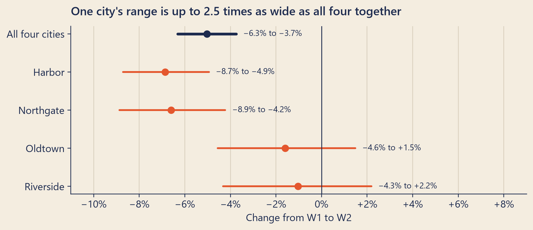
The 95% range for the real fall is −6.3% to −3.7%. A formula that treats the weekly counts as pure chance gives almost the same: −6.3% to −3.8%.
Be clear about what this range covers. It covers one kind of chance: which customers happened to order, and how often. It does not cover things that move every customer at once, such as rain or a holiday. Some shared causes have names, like rain. Others do not. In the summer, whole weeks missed the recipe by 0.85% (standard deviation), nearly twice the 0.48% that customer luck alone gives a week. So this range understates how much a whole week can wobble. Chapter 18 uses those summer weeks as a ruler: the spread of surprises in ordinary weeks, against which it judges one week.
Half the width of a range is its margin of error. For the fall it is about ± 1.3 points.
Now split the same fall by city:
Show the code
rows = [("All four cities", n_customers, fall_change, fall_lo, fall_hi)] +\ [(CITY[c], *by_city[c]) for c in CITY]fig, ax = bk.figure(8, 3.4)for y, (label, n, est, lo, hi) inenumerate(rows): color = bk.INK if y ==0else bk.TOMATO ax.plot([100* lo, 100* hi], [y, y], color=color, lw=3if y ==0else2, solid_capstyle="round") ax.scatter([100* est], [y], color=color, s=50, zorder=3) ax.text(100* hi +0.3, y, f"{span(lo, hi, pct)}", va="center", fontsize=9)ax.axvline(0, color=bk.INK, lw=0.9)ax.set_yticks(range(len(rows)), [r[0] for r in rows])ax.invert_yaxis()ax.grid(axis="y", visible=False)ax.grid(axis="x", color=bk.GRID)ax.set_xlim(-11, 9)ax.xaxis.set_major_locator(mticker.MultipleLocator(2))ax.xaxis.set_major_formatter(mticker.FuncFormatter(lambda v, _: "0%"ifround(v) ==0elsef"{v:+.0f}%".replace("-", "−")))ax.set_xlabel("Change from W1 to W2")ax.set_title(f"One city's range is up to {widest_ratio:.1f} times as wide as all four together")plt.show()
Figure 3: The change in completed orders from W1 to W2 (final statuses), with 95% ranges from resampling customers: all four cities together, and each city alone.
The all-cities range is 2.6 points wide. Riverside’s is 2.5 times as wide, with only about 15% of the customers: close to the 2.6 times that the square-root rule predicts. One city alone is a small spoonful. That is why Chapter 16 did not lean on any single city, and leaned instead on all four pointing the same way.
A range for a difference
The fall is itself a difference: W2 compared with W1. Both weeks carry their own luck, and a difference collects the luck of both sides. When the two sides are independent, the noise does not add up directly; it adds up in squares:
SE of a difference = √(SE of the first² + SE of the second²).
When the two parts are independent, a difference is noisier than either part. If two weeks each have an SE of 1, their difference has an SE of about 1.4, not 2 and not 0.
This leads to a common mistake. People draw two ranges, see that they overlap, and decide that the difference “is not real”. Overlap is the wrong test. Two 95% ranges can overlap a little while their difference is still clear. To judge a difference, build a range for the difference itself, or test it (Chapter 18).
NoteUnder the hood
A difference. If \(\hat a\) and \(\hat b\) are independent, \(\operatorname{Var}(\hat a - \hat b) = \operatorname{Var}(\hat a) + \operatorname{Var}(\hat b)\), so
\[\operatorname{SE}(\hat a - \hat b) = \sqrt{\operatorname{SE}(\hat a)^2 + \operatorname{SE}(\hat b)^2}.\]
If they are positively linked, subtract twice the covariance: the same customers in both weeks make a week-over-week change less noisy than two unrelated weeks would be.
A ratio of counts. For counts \(O_1\) and \(O_2\) that behave like Poisson counts, \(\operatorname{Var}(\log O) \approx 1/O\), so
With \(O_1\) = 45,441 and \(O_2\) = 43,153, that is 0.0067. The range is \(\frac{O_2}{O_1} e^{\pm 1.96 \cdot \text{SE}} - 1\). The customer bootstrap needs no Poisson assumption; that the two agree says the counts behave close to Poisson.
Square-root law. Most standard errors are proportional to \(1/\sqrt{n}\). One city with a fraction \(f\) of the data has a range about \(1/\sqrt{f}\) times as wide. The recipe shows it too. Fitted on August alone, the last four summer weeks, it puts the rain at 3.3 points, with a range from 2.7 to 4.2: 2.8 times as wide as the full summer’s. August has less than a third as many city-days, and only 17 rainy ones against 79. Rainy days are what teach the recipe about rain, and the rule on rainy days predicts √(79/17) ≈ 2.2 times as wide; the rest is the wobble of a small sample.
Overlap. Two independent 95% intervals of equal width \(\pm m\) do not overlap only when the estimates differ by more than \(2m\). But the difference is already significant at the 5% level when the estimates differ by more than \(\sqrt 2\, m\) ≈ \(1.41m\). Between those two gaps, the intervals overlap and the difference is still clear (Cumming and Finch, 2005).
Ranges for the board
At four o’clock, Mia rewrote Friday’s page. Every number now had a range, and a note on what the range covered.
Piece
Points
95% range
What the range covers
Tracking bug (Chapter 15)
7.0
none needed
Nothing to cover: it answers ‘what happened in these weeks?’
Rainy week before (Chapter 16)
3.4
3.1 to 3.7
Which summer days the recipe learned from (days and weeks resampled)
Normal weekly growth (Chapter 16)
−0.3
−0.4 to −0.1
The same resamples
Explained so far
10.1
9.8 to 10.4
The same resamples; the bug is a count
She added three rules at the bottom of the page, for herself as much as for Dana.
Say the range with the number, every time. “About 3.4 points, with a 95% range of 3.1 to 3.7” is one sentence. A number without a range invites the listener to imagine one, and people imagine ranges that are too narrow.
Round to what the range supports. A range from 3.1 to 3.7 points does not support two decimals. “3.39” sounds precise, and it is not.
Say what the range does not cover. The rain’s range assumes the recipe is right: that rain in early September works like rain in the summer. The range measures the luck of the data, not mistakes in the recipe. A recipe that left out a cause would be wrong by an amount no bootstrap can see.
There was one number she did not put a range on: the last 1.9 points. They are what is left after everything else, so their range collects the wobble of every other number, including the luck of the week itself. And the question Dana would ask about them is a different one. Not “how big is it?” but “is it there at all, or is it the miss of an ordinary week?” That question has its own tool (Chapter 18).
Common traps
“There is a 95% chance the truth is in my interval.” The 95% belongs to the method. Say: “a range built by a method that catches the true value 95 times in 100.”
Mixing up SD and SE. The SD describes single values; the SE describes an estimate. Reporting the SD of daily orders as the “uncertainty” of a weekly average makes it look far less certain than it is. The reverse makes it look far more certain.
Treating linked data as independent. Days in a wet spell, orders from one customer, users in one city: if units are linked, resample them in blocks or at the higher level, or the range comes out too narrow.
Reading overlap as “no difference”. Build a range for the difference instead.
Believing the range covers every mistake. It covers the luck of the sample. A biased sample, a wrong definition or a recipe that misses a cause can all be wrong by more than the range, and the range will not warn you.
Too many digits. Round to what the range supports.
TipAudit Instinct · Sampling risk and an honest limit
Mia’s habit of putting a range on every number came from audit sampling. ISA 530, the standard on audit sampling, separates two risks. Sampling risk is the risk that the conclusion from a sample differs from the conclusion the auditor would reach by testing the whole population. Non-sampling risk is everything else: the wrong procedure, a misread document, a population that was not complete.
When an auditor uses statistical sampling, with items chosen at random and probability theory to read the results, she can measure sampling risk. She projects the errors found in the sample to the whole population, then adds an allowance for sampling risk. The result is often stated as an upper limit at a chosen confidence, for example: “we are 95% confident that the misstatement is below $X.” (“95% confident” is shorthand: the 95% describes the method, not this one limit. Hoekstra and colleagues count reading it as a probability about one interval among the common misreadings.) If \(X\) is below tolerable misstatement, the most error she can accept, the sample supports the balance.
That sentence has the same parts as Mia’s: an estimate, a range, a confidence level, and a clear statement of what is covered. The bootstrap measures sampling risk. Non-sampling risk, such as a recipe that misses a cause, needs a different kind of check: the auditor’s judgement, and evidence from another direction.
NoteInterview Corner
1. Explain a 95% confidence interval to a non-technical manager.
NoteA short answer
“Our best estimate is 3.4 points, and the range is 3.1 to 3.7. We built the range with a method that, used again and again on new data, contains the true value about 95 times in 100. The range covers the luck of which days we happened to observe; it does not cover a mistake in our model.” Avoid saying “95% chance the true value is in this range”: the 95% describes the method.
2. What is the difference between standard deviation and standard error?
NoteA short answer
The standard deviation describes how spread out single values are, for example how much one day’s orders differ from another’s. The standard error describes how much an estimate, such as an average or a regression coefficient, would vary from sample to sample. For an average of \(n\) independent values, SE = SD / √n. The SD stays about the same as you collect more data; the SE shrinks.
3. When would you use the bootstrap?
NoteA short answer
When there is no simple formula for the standard error, or when I do not trust the formula’s assumptions: medians, ratios, percentiles, the output of a model, or a multi-step number like “points explained by rain”. Resample the units that are independent: users rather than orders, or whole blocks of time when days are linked. Use enough resamples (a few thousand for an interval). Be careful with very small samples and with extreme values such as maxima, where the bootstrap does poorly.
Ranges Dana can say
Dana read the new page standing up.
“‘Rain explains about 3.4 points, with a 95% range of 3.1 to 3.7,’” she read aloud. “I can say that.” She looked down the table. “And the bug has no range.”
“The bug’s 7.0 points answer the question ‘what happened in these weeks?’” said Mia. “The dashboard missed those orders. That is a fact, so it needs no range. The fall answers a different question: what would a rerun of these weeks give? A rerun would have new luck, so that answer needs a range.”
“And these last 1.9 points?”
“They need a different question,” said Mia. “Not how big they are, but whether they are there at all. I will start on it tomorrow.”
Theo did not look up from his screen. “I will bring the doubts.”
Reported change: −12.0% orders, the week of 7 September compared with the week before (CEO dashboard).
Explained so far: 10.1 of the 12 points (95% range 9.8 to 10.4). The tracking bug, 7.0, a count that needs no range (Chapter 15); the rainy week before, 3.4 (range 3.1 to 3.7); normal growth, −0.3 (range −0.4 to −0.1) (Chapter 16).
Suspects: something real on or after 7 September that lowered orders in every city, or luck in W1 that did not repeat. Not proved; not named yet.
Ruled out: the matcha menu (Chapter 4); every stop on the data’s journey after the app (Chapters 8–14).
Open questions: Is the last 1.9 points more than a normal week’s miss? (Chapter 18.) Why did drinks per order fall after 7 September? (Chapter 21.)
New evidence: ranges for every estimated number, from bootstraps of the summer (days and weeks) and of customers. Completed orders fell −5.0% (finance’s definition, final statuses), 95% range −6.3% to −3.7% from customer luck alone.
Recap
The standard deviation describes single values; the standard error describes an estimate. For an average, SE = SD ÷ √n.
The bootstrap measures uncertainty by resampling your own data, many times. Resample the units that are truly independent: customers rather than orders, whole weeks when days are linked.
A 95% interval comes from a method that catches the truth 95 times in 100. Report it with every estimate, round to what it supports, and say what it does not cover. Rain: 3.4 points, range 3.1 to 3.7.
English
中文
standard deviation (SD)
标准差
standard error (SE)
标准误
confidence interval
置信区间
confidence level
置信水平
bootstrap
自助法
resample
重抽样
with replacement
有放回
block bootstrap
区组自助法 / 块自助法
independent
独立
margin of error
误差范围
percentile
百分位数
sampling risk
抽样风险
non-sampling risk
非抽样风险
tolerable misstatement
可容忍错报
Further reading
Efron, B. (1979). Bootstrap Methods: Another Look at the Jackknife. The Annals of Statistics, 7(1), 1–26. doi:10.1214/aos/1176344552. The paper that introduced the bootstrap.
Künsch, H. R. (1989). The Jackknife and the Bootstrap for General Stationary Observations. The Annals of Statistics, 17(3), 1217–1241. doi:10.1214/aos/1176347265. The block bootstrap with overlapping blocks, for data that are linked over time.
Carlstein, E. (1986). The Use of Subseries Values for Estimating the Variance of a General Statistic from a Stationary Sequence. The Annals of Statistics, 14(3). doi:10.1214/aos/1176350057. Non-overlapping blocks, like Mia’s weeks.
Neyman, J. (1937). Outline of a Theory of Statistical Estimation Based on the Classical Theory of Probability. Philosophical Transactions of the Royal Society of London. Series A, 236(767), 333–380. doi:10.1098/rsta.1937.0005. Where confidence intervals come from.
Cumming, G., & Finch, S. (2005). Inference by Eye: Confidence Intervals and How to Read Pictures of Data. American Psychologist, 60(2), 170–180. doi:10.1037/0003-066X.60.2.170. Includes the rule for reading two overlapping intervals.
Hoekstra, R., Morey, R. D., Rouder, J. N., & Wagenmakers, E.-J. (2014). Robust misinterpretation of confidence intervals. Psychonomic Bulletin & Review, 21(5), 1157–1164. doi:10.3758/s13423-013-0572-3. Researchers and students misread intervals in the same ways; a useful warning.
International Auditing and Assurance Standards Board. ISA 530, Audit Sampling. IAASB Handbook, 2012 edition (PDF). Paragraph 5 defines sampling risk and non-sampling risk.