16 · Randomness Has a Shape
On Friday morning, Mia opened a table she had never needed before: weather. It had one row for each city and each day since 1 June. One column held the rain in millimetres. Another, is_rainy, said yes or no: yes meant at least 1 mm of rain that day.
Yesterday’s last question was still at the top of her notebook. Dana had asked it: The rain?
Priya Nair, the product manager, stopped at Mia’s desk with a cup of tea. “I said it on the first day,” she said. “It rained all through the week before the drop. Then the sun came out, and people walked to the shop instead of ordering.”
“Maybe,” said Mia. “How many orders does a rainy day add?”
Priya thought about it. “A lot?”
Theo looked up from the next desk. “‘A lot’ is not a unit.”
Mia wrote two lines in her notebook.
Completed orders (finance’s definition): down about 5%, W2 against W1. A normal week: ?
In her notes, W1 is the week before the drop, 31 August to 6 September, and W2 is the week of the drop, 7 September to 13 September. (This book’s headline numbers use final statuses, see Chapter 1: −5.0%.) The first line was solid now. Chapter 15 had shown that the dashboard’s other 7.0 points were a tracking bug. The second line was the problem. “Week over week” compares one week with one other week. If that other week was unusual, the comparison is unfair. The counting can be right and the comparison still unfair.
So Mia asked a different question. Not “how did W2 compare with W1?” but “how did W2 compare with what a normal week would have looked like?” To answer it, she first had to learn what normal looks like: how much a normal week wobbles, which patterns repeat, and what rain does.
ImportantThe big idea
Before you call a change real, build an expectation of what a normal week would look like. Then measure the change against that expectation, not against one other week.
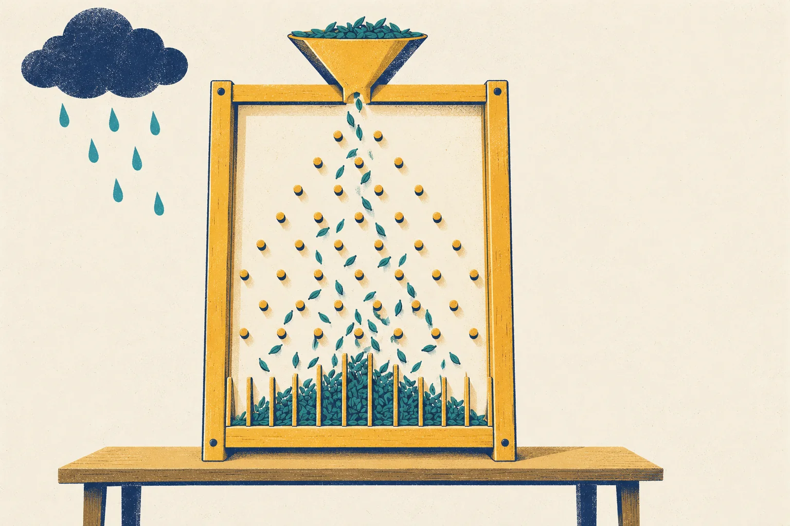
Look at the board in the picture. Every leaf falls through the same pegs, yet each one lands in a different slot. You cannot say where one leaf will land. But pour in thousands, and the piles always take the same shape: high in the middle, low at the sides. Single events are random. Many events together have a shape you can learn. The rain cloud in the corner is the other half of the chapter: a cause that pushes many leaves the same way.
A spoonful of soup
A cook does not eat the whole pot to know if the soup needs salt. She tastes one spoonful. The pot is the population: everything you want to know about. The spoonful is the sample: the part you really look at. One spoonful is enough if the soup is well stirred, so that every part of the pot had the same chance to end up in the spoon. That is a random sample.
Steep’s summer is a good pot to practise on. From 1 June to 30 August, Steep had 565,050 completed orders. Mia can count all of them, so she knows the true answer to a simple question: Harbor’s share of the orders was 40.1%. Because the truth is known, you can taste spoonfuls and see how close they come.
Things to try:
- Set the spoonful to 10. The share can only be 0%, 10%, 20% and so on, and it is often far from the truth.
- Move up to 100, then 1,000, then 10,000. Watch the pile get narrower each time.
- Press “Stir and taste again” a few times and watch the top line. Its start changes every time. Its end does not.
The top line wanders a lot at first. After ten orders it can be anywhere. After a thousand it is close to the dashed line, and after ten thousand it hardly moves. This is the law of large numbers: as a random sample grows, its average, or its share, gets closer and closer to the true value of the population.
Two warnings come with the law. First, it says nothing about small samples. They can be far off. Second, the early luck is not cancelled. If the first ten orders were all from Harbor, the next ten are not more likely to come from elsewhere. The early luck is only diluted: it becomes a smaller part of a bigger total.
The random ups and downs in each spoonful have a name: noise. Noise is variation with no single cause you can point to. Here, it is only the luck of which orders happened to land in the spoon.
There is a twist that matters for the rest of this book. The summer itself is a spoonful. When Mia asks “what does a normal Tuesday look like?”, the pot is every Tuesday that could have happened, and the summer gave her only thirteen of them. Everything she learns from the summer is a sample, so it comes with noise. Chapter 17 measures how much.
Noise has a shape
Set the spoonful to 100 and look at the pile in the playground. Most spoonfuls land near the truth. Fewer land far away, and almost none land very far away. Piled up, they make a hill: highest in the middle, falling away evenly on both sides. This is the bell shape. The smooth curve that describes it is called the normal distribution.
The bell usually appears when a result is the sum of many small, separate bits of luck, and no single bit is big. That is what happens to each leaf in the opener picture: every peg pushes it a little to the left or a little to the right. Most leaves get about as many pushes one way as the other, and land near the middle. A few get many pushes the same way, and land at the edges.
To say how wide a bell is, you need a measure of spread. The variance is the average squared distance of the values from their average. Squaring makes every distance positive, and it makes big distances count more. Its square root is the standard deviation (SD), which is back in the original units, such as orders or percentage points. For a bell shape, a useful rule is:
- about two values in three lie within 1 SD of the middle, and
- about 95 in 100 lie within 2 SDs.
For spoonfuls of 100 orders, the SD of Harbor’s share is about 4.9 points. For spoonfuls of 1,000, it is about 1.5. Ten times more data gives about a third of the noise, not a tenth. The noise shrinks with the square root of the sample size: four times the data, half the noise.
NoteUnder the hood
For values \(x_1, \dots, x_n\) with average \(\bar x\), the sample variance and standard deviation are
\[s^2 = \frac{1}{n-1}\sum_{i=1}^{n} (x_i - \bar x)^2,\]
\[s = \sqrt{s^2}.\]
(Dividing by \(n - 1\) instead of \(n\) corrects a small bias: the values sit a little closer to their own average than to the true mean.)
A spoonful of \(n\) orders from a pot where a share \(p\) comes from Harbor gives a sample share \(\hat p\). Its average is \(p\), and its standard deviation is
\[\operatorname{SD}(\hat p) = \sqrt{\frac{p(1-p)}{n}}.\]
With \(p\) = 0.401, that is 0.155 for \(n = 10\), 0.049 for \(n = 100\) and 0.0049 for \(n = 10{,}000\). The playground draws with replacement, which is the same as tasting a tiny part of a very large pot.
The law of large numbers says that \(\hat p \to p\) as \(n\) grows. The central limit theorem says more: for large \(n\), the distribution of \(\hat p\) (and of most averages) is close to a normal distribution with this standard deviation. That is why the pile in the playground looks like a bell. With \(n = 10\) the pile is lumpy and not yet a good bell; the theorem is a statement about large \(n\).
What a normal week looks like
Mia’s next step was to look at a normal summer. She started with Harbor, the biggest city, and drew every day from 1 June to the end of the week of the drop.
Show the code
harbor = city_day[city_day.city == "harbor"]
bk.setup()
fig, ax = bk.figure(8, 3.9)
for start, end, label in [(W1_START, W1_END, "W1"), (W2_START, W2_END, "W2")]:
    ax.axvspan(start - pd.Timedelta(hours=12), end + pd.Timedelta(hours=12),
               color=bk.TEAL if label == "W1" else bk.TOMATO, alpha=0.12, lw=0)
    ax.text(start + pd.Timedelta(days=3), harbor.orders.max() * 1.05, label, ha="center", fontsize=10,
            color=bk.TEAL_TEXT if label == "W1" else bk.TOMATO_TEXT)
ax.plot(harbor.day, harbor.orders, color=bk.INK, lw=1.3)
wet = harbor[harbor.is_rainy]
ax.scatter(wet.day, wet.orders, s=30, color=bk.TEAL, zorder=3, label="rainy day")
ax.legend(loc="lower right", fontsize=9)
ax.set_ylim(harbor.orders.min() * 0.92, harbor.orders.max() * 1.1)
ax.set_ylabel("Orders per day")
ax.xaxis.set_major_locator(mdates.MonthLocator())
ax.xaxis.set_major_formatter(mdates.DateFormatter("%b"))
ax.set_title("Harbor: the same weekly rhythm, slow growth, and jumps on rainy days")
plt.show()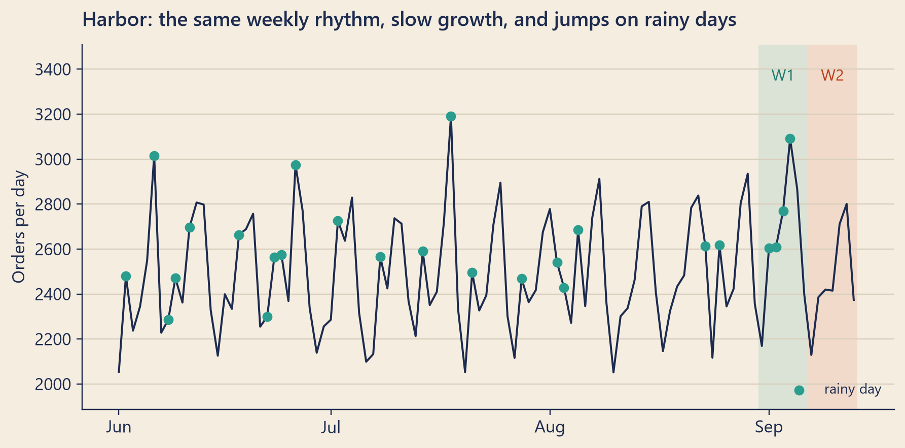
Three patterns stand out, plus a fourth thing that is not a pattern at all.
- A weekly rhythm. Every week has the same shape. Across all four cities, an average summer Monday had 5,462 orders and an average Saturday 7,126, about 30% more. A pattern that repeats with the calendar is called seasonality. Steep has a weekly one. It may also have a yearly one, with more tea in winter than in summer, but thirteen summer weeks cannot show that.
- Slow growth. The line drifts upward. A slow, steady movement in one direction is a trend.
- Rain. The teal dots, the rainy days, mostly sit above the usual level for their weekday.
- Noise. Even two dry Tuesdays a week apart are not the same. What is left after the patterns is noise.
Weekly totals hide the first pattern, because every week has exactly one of each weekday. So the fair way to compare weeks is whole weeks: Monday to Sunday, as Steep’s weeks run. Mia added up the thirteen summer weeks and looked at the twelve changes from one week to the next.
Show the code
changes = weekly.orders.pct_change().loc[1: w2_week]
labels = [f"{d:%d %b}" for d in weekly.start.loc[1: w2_week]]
colors = [bk.MUTED] * (len(changes) - 2) + [bk.TEAL, bk.TOMATO]
fig, ax = bk.figure(8, 3.9)
ax.bar(range(len(changes)), 100 * changes, color=colors, width=0.7)
ax.axhline(0, color=bk.INK, lw=0.9)
for edge in (1, -1):
    ax.axhline(100 * edge * summer_changes.abs().max(), color=bk.INK, ls=":", lw=0.9)
ax.text(len(changes) - 0.5, 100 * true_change, f" {pct(true_change)}", va="center", fontsize=10,
        color=bk.TOMATO_TEXT)
ax.set_xticks(range(len(changes)), labels, rotation=90, fontsize=8)
ax.set_xlabel("Week starting")
ax.set_ylabel("Change from the week before (%)")
ax.set_xlim(-0.6, len(changes) + 0.9)
ax.yaxis.set_major_formatter(mticker.FuncFormatter(lambda v, _: f"{v:.0f}%".replace("-", "−")))
ax.set_title(f"A fall of {bk.fmt_pct(-true_change)} was bigger than any change this summer")
plt.show()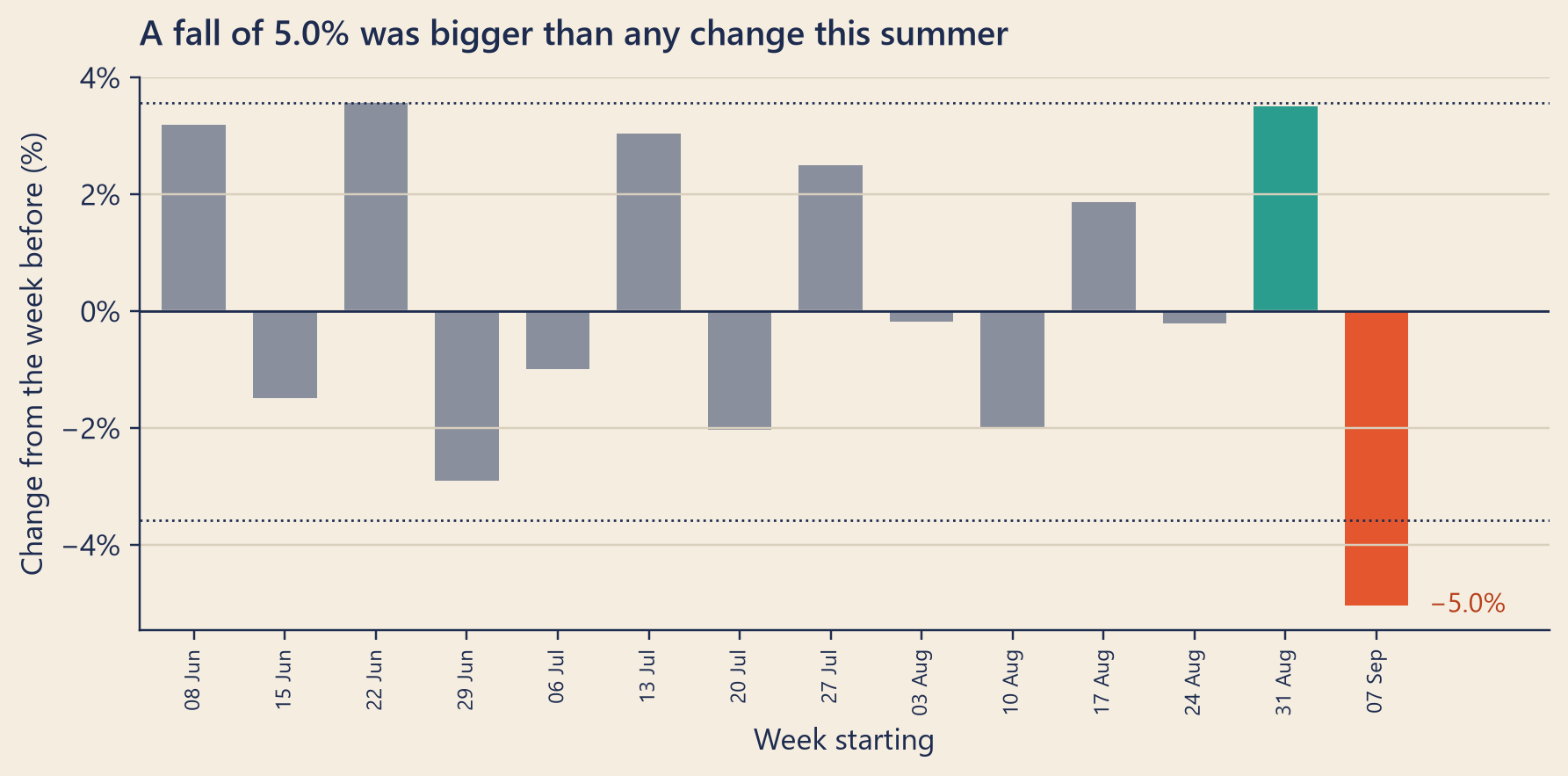
Over the summer, the typical week-to-week change had a standard deviation of 2.3%. The biggest rise was +3.6% and the biggest fall −2.9%. The fall that Dana’s question was about, −5.0%, is bigger than all of them.
“So it is real,” said Priya. “Bigger than anything all summer.”
“Bigger than any change all summer,” said Mia. “But a change compares two weeks. Look at the bar before it.” The week before the drop, W1, had risen +3.5%. With 45,441 orders, it was the busiest week since 1 June. A fall from the busiest week is a fall from an unusual height.
A third thing behind both
Across the summer, 22% of the city-days were rainy. (A city-day is one city on one day, so the summer has 364 of them.) Rain keeps people indoors, and people indoors order tea. Mia made the simplest fair comparison she could: in each city, she compared the rainy days with the dry days of the same weekday. On average, the rainy days had 11% more orders.
Then she looked at the two weeks in question. In W1, it rained in Harbor, Tuesday to Friday; Northgate, Thursday and Friday. In W2 it did not rain anywhere, not for a single city-day.
This is a confounder, the idea from Chapter 4: a third thing that affects both the groups you compare and the result you measure. There, the city decided which stores got the matcha menu, and also how well they converted. Here, the two “groups” are two weeks. The weather was different in them, and the weather moves orders. A plain comparison of W2 with W1 mixes two stories: what changed at Steep, and what changed in the sky.
The cities show it clearly. Chapter 5 left a question open: why did the two big cities fall more? Here are the falls:
| City | Rain in W1 | Change, W2 vs W1 |
|---|---|---|
| Harbor | Tuesday to Friday | −6.9% |
| Northgate | Thursday and Friday | −6.6% |
| Oldtown | none | −1.6% |
| Riverside | none | −1.0% |
The two cities that fell most are the two where it rained in W1. The rain also explains the false alarms of Chapter 15’s volume test. That test compared each day with the same weekday a week earlier, and in the summer it failed only a week after rain. Against a rainy day, a normal dry day looks like a fall.
Why a record week is followed by a quieter one
Rain made W1 busy. But there is a general reason why a busy week is usually followed by a quieter one, whatever made it busy. Mia looked for it in the summer. She took the three busiest summer weeks and looked at the week after each one:
- The three busiest weeks averaged 44,206 orders. The weeks right after them averaged 43,455.
- The three quietest weeks averaged 42,562. The weeks right after them averaged 43,954.
- The average summer week had 43,465.
Every busy week was followed by a quieter one, and every quiet week by a busier one. The weeks after landed much closer to the summer average.
This is regression to the mean. When a result is partly luck, an extreme result is usually followed by a more ordinary one, because the luck does not repeat. Nothing pulls the second week back. It gets its own, new luck, and new luck is usually average.
In Steep’s summer, most of this luck was weather. The busiest weeks were busy because of rain. Rain added 2.6% to 5.8% to them. Without the rain, they were normal: within 0.7% of a normal week. (The next section shows how Mia measured that.) Steep cannot control rain, so for Steep, rain is luck. And a wet week is rarely followed by another wet one. The wettest summer week, from 22 June, had 14 rainy city-days and was the busiest week of the summer. The week after it fell 2.9%.
Regression to the mean fools people because it looks like a cause. A store has its worst week, the manager sends a stern email, and the next week is better. The email gets the credit, though the next week would probably have been better anyway. The idea is old. Francis Galton described it in 1886, using the heights of parents and their children. The board in the opener picture is named after him: a Galton board. He built one to show how many small pushes make a bell.
NoteUnder the hood
Write each week’s total as a steady level plus luck: \(Y_t = \mu + \varepsilon_t\), where the \(\varepsilon_t\) are independent, with mean 0. If week \(t\) is far above \(\mu\), the best guess for week \(t+1\) is still \(\mu\), because \(\varepsilon_{t+1}\) knows nothing about \(\varepsilon_t\).
More generally, if a measured value is a true value plus noise, \(X = T + \varepsilon\), then the best guess for the true value given the measurement is
\[E[T \mid X] = \mu + \rho\,(X - \mu),\]
\[\rho = \frac{\operatorname{Var}(T)}{\operatorname{Var}(T) + \operatorname{Var}(\varepsilon)},\]
when \(T\) and \(\varepsilon\) are normal. Because \(\rho < 1\), the guess sits closer to the average than the measurement did. The more of the variation is noise, the stronger the pull.
A side effect: week-to-week changes of such a series tend to alternate. A lucky week makes the change into it big and the change out of it small. In the summer, the correlation between one week’s change and the next was −0.66; for pure noise around a fixed level, it would be −0.5.
A recipe for a normal day
Mia now had the ingredients of a normal day: the city, the weekday, the rain and the date. What she needed was a way to put them together, to say how many orders a normal day should bring. She wrote it in her notebook as a recipe card.
A recipe for a normal day
- Start with the city’s usual level.
- Multiply by the weekday’s factor.
- If it rains, multiply by the rain factor.
- Multiply by the growth since 1 June.
The numbers on the card are not guesses. The recipe learns them from the summer: 364 city-days, from 1 June to 30 August. It learns them in the way that makes its predictions closest to what really happened, on the whole. Note the dates: the recipe learns only from days before W1. It has never seen the two weeks it will judge, so it cannot learn their answer by heart.
Here is what it learned:
- Rain multiplies a city-day’s orders by 1.113: about 11.3% more.
- Weekdays: Monday is the quietest day. Saturday is the busiest, at 1.31 times a Monday.
- Growth: about +0.29% per week.
And here is the card at work on a real day: Harbor, Friday 4 September, a rainy day in W1.
| Step | Factor | Running total |
|---|---|---|
| Harbor’s usual level (a dry Monday on 1 June) | 2,099 | |
| It is a Friday | × 1.268 | 2,661 |
| It rains | × 1.113 | 2,961 |
| 95 days of growth | × 1.040 | 3,078 |
That day, Harbor really had 3,091 orders. The recipe’s guess for a day is called the expectation, or expected value: what a normal day like this one should bring, on average.
Is the recipe any good? Mia checked it on whole weeks: she added up what it expected for each week and put it next to what really happened.
Show the code
shown = weekly.loc[:w2_week]
fig, ax = bk.figure(8, 3.8)
ax.axvspan(w1_week - 0.5, w2_week + 0.5, color=bk.GRID, alpha=0.45, lw=0)
ax.text((w1_week + w2_week) / 2, shown.orders.max() * 1.012, "W1, W2", ha="center", fontsize=9)
ax.plot(shown.index, shown.expected, color=bk.MUSTARD, lw=2.6, marker="o", ms=5, label="the recipe expected")
ax.plot(shown.index, shown.orders, color=bk.INK, lw=1.8, marker="o", ms=4, label="what happened")
ax.legend(loc="lower right", fontsize=9)
ax.set_xticks(shown.index, [f"{d:%d %b}" for d in shown.start], rotation=90, fontsize=8)
ax.set_xlabel("Week starting")
ax.set_ylabel("Orders per week")
ax.yaxis.set_major_formatter(mticker.FuncFormatter(lambda v, _: f"{v:,.0f}"))
ax.set_ylim(shown.orders.min() * 0.97, shown.orders.max() * 1.03)
ax.set_title("The recipe follows the summer's ups and downs")
plt.show()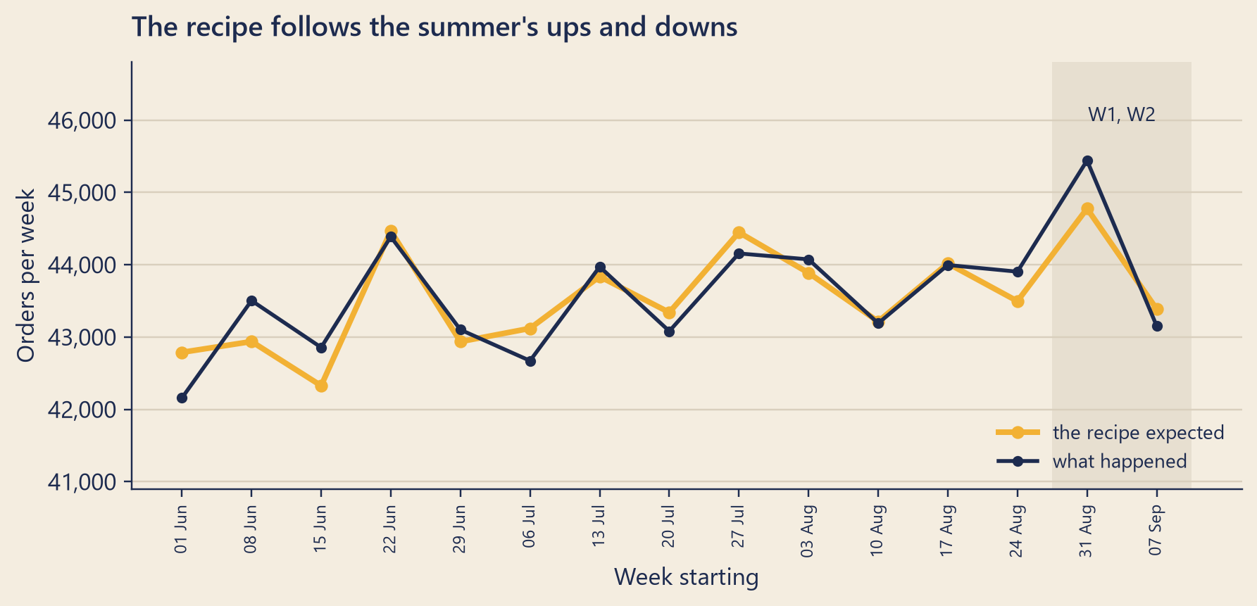
The recipe follows the summer closely. When a wet week pushed orders up, the recipe expected it, because it knew about the rain. It is not perfect, and it is not meant to be: the noise is still there.
What is left over has a shape too. For every summer city-day, Mia took the miss: how far the real orders were from the recipe, in percent.
Show the code
fig, ax = bk.figure(8, 3.4)
ax.hist(100 * summer.miss, bins=np.arange(-12, 12.5, 1), color=bk.TOMATO, edgecolor=bk.PAPER, lw=0.6)
for edge in (-2, 2):
    ax.axvline(100 * edge * miss_sd, color=bk.INK, ls="--", lw=1)
ax.set_xlabel("Real orders compared with the recipe (%)")
ax.set_ylabel("City-days")
ax.xaxis.set_major_formatter(mticker.FuncFormatter(lambda v, _: "0%" if round(v) == 0 else f"{v:+.0f}%".replace("-", "−")))
ax.set_title("What the recipe cannot explain forms a bell")
plt.show()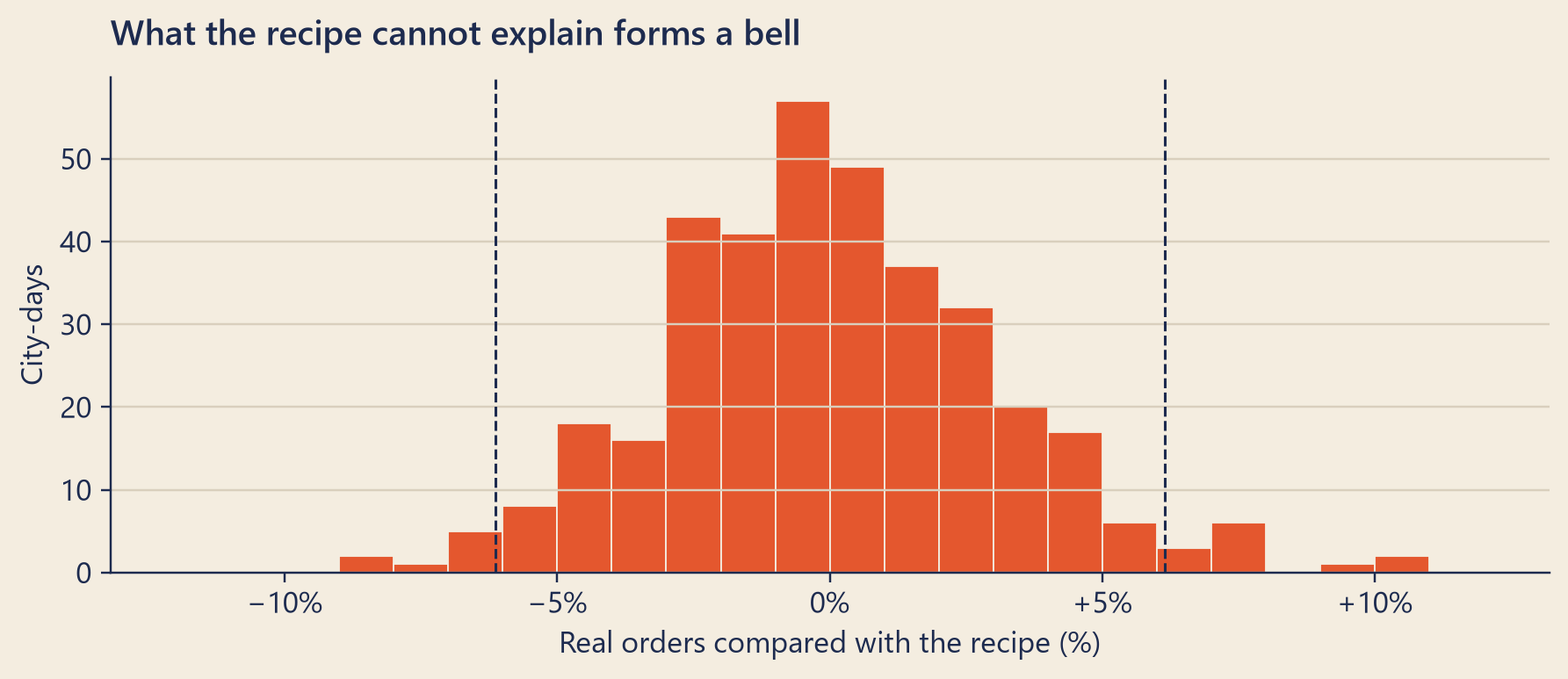
The misses form a bell around zero, with a standard deviation of 3.1%. In this data, 72% of them lie within 1 SD and 95% within 2 SDs, close to the rule of two in three and 95 in 100. This is the shape of randomness in Steep’s orders. Once the patterns you can explain are taken out, what is left behaves like the leaves on the board. That shape is what will let Mia say, with numbers, what “normal” means (Chapters 17 and 18).
NoteUnder the hood
The recipe is a linear regression on the logarithm of orders. For city \(c\) on day \(d\):
\[\begin{aligned} \log(\text{orders}_{c,d}) = {} & a_c + w_{\text{weekday}(d)} \\ & + r \cdot \text{rain}_{c,d} + g \cdot t_d + \varepsilon_{c,d}, \end{aligned}\]
where \(a_c\) is one level per city, \(w\) is one term for each weekday from Tuesday to Sunday (Monday is the base, \(w = 0\)), \(\text{rain}_{c,d}\) is 1 on a rainy city-day and 0 otherwise, \(t_d\) counts days since 1 June, and \(\varepsilon_{c,d}\) is the miss. Least squares chooses the twelve numbers that make the sum of the squared misses as small as possible, using the 364 summer city-days. In code, this is steep.metrics.weather_attribution, the same function Chapter 21 uses.
Taking the logarithm turns the recipe’s multiplications into additions, which is what a linear regression needs. Going back, each term becomes a factor: rain multiplies orders by \(e^{r}\) = 1.1126 (here \(r\) = 0.1067), and growth by \(e^{7g}\) = 1.0029 per week. The miss \(\varepsilon\) has a standard deviation of about 0.031 on the log scale, which is about 3.1%.
The expected orders for a city-day are \(\exp(\hat a_c + \hat w + \hat r \cdot \text{rain} + \hat g t)\). Strictly, this is the median of a log-normal miss, not its mean. The mean is larger by a factor of \(e^{s^2/2}\) ≈ 1.0005. That factor is the same for every day, so it cancels in every ratio this chapter uses.
The expected week
Now Mia could do what she came for. She ran the recipe on W1 and W2, twice.
- With no rain anywhere, the recipe expects W2 to be +0.3% against W1. That is one week of normal growth. W2 is W1 moved seven days later, with the same cities and the same weekdays, so growth is the only difference left.
- With the real rain, the recipe expects −3.1%. W1 had six rainy city-days and W2 had none, so a normal W2 should be lower than W1.
- What happened to completed orders: −5.0% (finance’s definition, final statuses).
Show the code
days = city_day[in_w1 | in_w2].groupby("day")[["orders", "expected", "expected_dry"]].sum()
fig, ax = bk.figure(8, 3.9)
x = np.arange(len(days))
ax.bar(x, days.orders, color=[bk.TEAL] * 7 + [bk.TOMATO] * 7, width=0.7, label="what happened")
ax.scatter(x, days.expected, color=bk.INK, s=34, zorder=3, label="recipe, real rain")
ax.scatter(x, days.expected_dry, facecolor="none", edgecolor=bk.INK, s=60, lw=1.2, zorder=3,
           label="recipe, no rain")
ax.set_xticks(x, [f"{d:%a}\n{d.day} {d:%b}" for d in days.index], fontsize=8)
ax.set_ylim(0, days[["orders", "expected"]].max().max() * 1.16)
ax.set_ylabel("Orders per day")
ax.yaxis.set_major_formatter(mticker.FuncFormatter(lambda v, _: f"{v:,.0f}"))
ax.legend(loc="upper left", fontsize=8, ncols=3)
ax.set_title("The recipe expected W1's rainy days to be busy")
plt.show()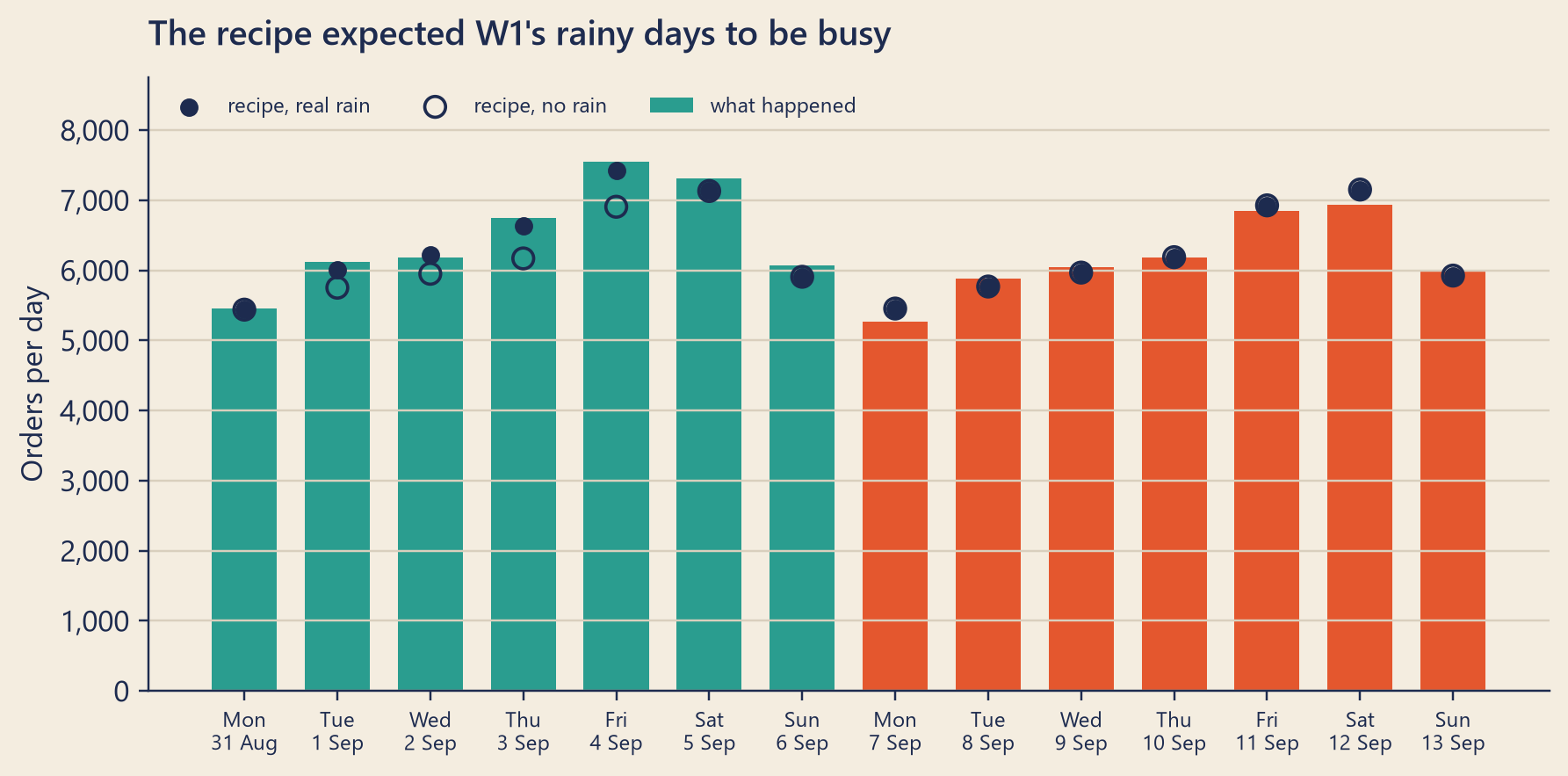
The difference between the two expected changes is the part of the fall that rain explains: 3.4 points. Growth works the other way. A normal W2 should be slightly above W1, so growth makes the gap 0.3 points bigger, not smaller. Mia wrote the ledger:
| Piece | Points of the 12 |
|---|---|
| Tracking bug (Chapter 15) | 7.0 |
| Rainy week before, dry week after | 3.4 |
| Normal weekly growth, which pushes the other way | −0.3 |
| Explained so far | 10.1 |
| Still open: W2 fell further from W1 than the recipe expected | 1.9 |
W1 also had luck of its own. Even after its rain, it was 1.5% above the recipe, further above it than any summer week had been. W2 was 0.5% below. Part of the 1.9 points still open may be W1’s luck, which did not repeat. Chapter 18 tests this.
Try it: make it rain
Every square below is one city on one day. Click a square to add or remove rain, and watch what the recipe expects. “Real rain” puts back what really happened.
Bars: what the recipe expects with the rain you chose. Dots: what really happened.
Things to try:
- Press “No rain at all”. The recipe now expects a small rise, and the gap to what happened is much bigger.
- Put rain on all four cities on the Thursday of W2. How much of the fall disappears?
- Move W1’s Harbor rain to Riverside, square by square. Why does it explain less?
Moving rain from Harbor to Riverside explains less because the recipe multiplies: 11% more of Harbor’s orders is many more orders than 11% more of Riverside’s.
Mia looked at each city again, now against its own expectation:
| City | Expected change | Real change | Short by (points) | W1 against the recipe | W2 against the recipe |
|---|---|---|---|---|---|
| Harbor | −5.8% | −6.9% | 1.1 | +0.3% | −0.8% |
| Northgate | −3.0% | −6.6% | 3.6 | +3.4% | −0.5% |
| Oldtown | +0.3% | −1.6% | 1.9 | +1.3% | −0.7% |
| Riverside | +0.3% | −1.0% | 1.3 | +1.6% | +0.2% |
In every city, the change fell short of what the recipe expected. That includes Oldtown and Riverside, where it did not rain at all; there, the change fell 1.3 to 1.9 points short. The last two columns show where the gap sits. W1 came in above the recipe in every city. W2 came in below it in three cities, and a little above it in Riverside.
One city is a small spoonful, and Chapter 17 will show how wide one city’s range is. But all four point the same way. The recipe cannot tell whether W1 was unusually high or W2 unusually low. Chapter 18 asks whether the gap is bigger than a normal week’s miss.
Common traps
- Comparing with one other week. The baseline may be unusual. Compare with an expectation built from many weeks.
- Learning from the weeks you judge. If the recipe learns from W1 and W2, it partly learns their answer. Fit on the past; judge the new.
- Calling a fall after a record week a problem. It may be regression to the mean. Ask first whether the record was normal.
- Explaining noise with a story. Every week moves. Before you explain a movement, ask how big normal movements are.
- Forgetting the calendar. Weekday mix, holidays, paydays and weather are all confounders that live in the calendar. Compare whole weeks, or put them in the recipe.
- A recipe built on the wrong numbers. Mia built hers on the orders database, not the dashboard. A recipe learned from data with a bug learns the bug.
TipAudit Instinct · Substantive analytical procedures
Auditors have a formal version of Mia’s recipe. ISA 520, the international standard on analytical procedures, asks an auditor who uses them as evidence to do four things before looking at the result:
- Decide whether this kind of procedure suits the question.
- Check that the data behind the expectation are reliable.
- Build an expectation precise enough to reveal an error that matters.
- Decide how big a difference from the expectation is acceptable without further work.
If the recorded number differs from the expectation by more than that, the auditor must investigate: ask management, and then find evidence for the answer. A story from management is not enough on its own.
A store’s revenue is a classic case. The auditor predicts it from things that drive it, such as opening days, number of staff, or last year’s revenue per square metre. Then she compares the books with the prediction. She does not compare this year with last year and stop there.
Mia’s recipe follows the same steps. The drivers are the city, the weekday, the rain and the date. The data are the orders database, which Chapter 15 proved reliable, not the dashboard, which did not count every order. Step 4 is the one she has not done yet: how big a miss is normal? That is Chapter 18.
NoteInterview Corner
1. Revenue fell 8% week over week. How do you decide if it is real?
NoteA short answer
First check the measurement: definitions, data completeness, late data, any changed pipeline or app release. Then check the comparison. Look at how big week-over-week changes normally are, from many past weeks. Check the baseline week for anything unusual: holidays, weather, promotions, a record high. Better still, build an expectation for the week from its drivers (weekday mix, seasonality, trend, weather, marketing), fitted on past data, and compare the week with that. Only a difference that is large compared with normal misses is worth explaining. Then split it by segment to find where it lives.
2. What is regression to the mean?
NoteA short answer
When a measurement is partly luck, an extreme value is usually followed by a value closer to the average, because the luck does not repeat. It is not a force, and nothing “corrects” itself; the next measurement gets new luck. It matters because it looks like a cause. If you act after an extreme result, such as a terrible week or a bad branch, the next result will usually look better even if your action did nothing. The fix is a comparison group, or an expectation that does not assume the extreme will continue.
3. What is a confounder? Give an example.
NoteA short answer
A third variable that affects both the groups you compare and the outcome. If one week was rainy and the next dry, and rain raises orders, then rain confounds the week-over-week comparison: part of the change belongs to the weather. You handle it by comparing like with like, or by putting the confounder into a model of what you expect, as long as it was not itself caused by the change you study.
Clue 2
At five o’clock, Mia went to Dana’s office with one page.
“You asked about the rain,” she said. “Some of it was the rain. The week before the drop was unusually wet in our two biggest cities, and the week of the drop was completely dry. With that rain, and normal growth, a fair comparison expects orders to fall about 3.1%. They fell about 5%.”
“So Priya was right.”
“Partly. The rain explains 3.4 points. With the bug, and after growth takes back 0.3, that is 10.1 of the 12. About 1.9 points are still open, in every city, even the dry ones.”
Dana looked at the page. “And is that gap real?”
“That is the right question,” said Mia. “Every week misses the recipe a little. Next I need to know how big a normal miss is, and how sure I am about each of these numbers.”
Reported change: −12.0% orders, the week of 7 September compared with the week before (CEO dashboard).
Explained so far: 10.1 of the 12 points. The tracking bug, 7.0 (Chapter 15); the rainy week before (Harbor, Tuesday to Friday; Northgate, Thursday and Friday) against a dry week after, 3.4; normal growth, which pushes the other way, −0.3 (this chapter). Clue 2, the unfair comparison, is closed: the recipe expected −3.1%, and completed orders fell −5.0% (finance’s definition, final statuses).
Suspects: something real on or after 7 September that lowered orders in every city, or luck in W1 that did not repeat (W1 was 1.5% above the recipe). Not proved; not named yet.
Ruled out: the matcha menu (Chapter 4); every stop on the data’s journey after the app (Chapters 8–14).
Open questions: About 1.9 points remain: W2 fell further from W1 than the recipe expected. How sure is Mia about each number? (Chapter 17.) Is the last 1.9 more than a normal week’s miss? (Chapter 18.) Why did drinks per order fall after 7 September? (Chapter 21.)
New evidence: the weather table; a recipe for a normal day, fitted on the summer: rain × 1.113, growth +0.29% per week.
Recap
- One week compared with one other week is a weak test. Build an expectation of a normal week from what drives it, and compare with that.
- Noise has a shape. Random samples and the recipe’s misses form a bell, and the standard deviation says how wide it is. Bigger samples wobble less, by the square root of their size.
- Watch the calendar: weekdays, trends and rain repeat or recur, and an extreme week is usually followed by a more ordinary one. Here, rain explains 3.4 points and growth −0.3, so 10.1 of the 12 points are explained.
| English | 中文 |
|---|---|
| population | 总体 |
| sample | 样本 |
| random sample | 随机样本 |
| noise | 噪声 |
| law of large numbers | 大数定律 |
| bell shape / normal distribution | 钟形 / 正态分布 |
| variance | 方差 |
| standard deviation | 标准差 |
| seasonality | 季节性 |
| trend | 趋势 |
| regression to the mean | 均值回归 |
| confounder | 混杂因素 |
| expectation (expected value) | 预期值(统计学中称期望值) |
| linear regression | 线性回归 |
| least squares | 最小二乘法 |
| analytical procedures | 分析程序 |
Further reading
- Galton, F. (1886). Regression Towards Mediocrity in Hereditary Stature. The Journal of the Anthropological Institute of Great Britain and Ireland, 15, 246–263. doi:10.2307/2841583. Where the name “regression” comes from.
- Barnett, A. G., van der Pols, J. C., & Dobson, A. J. (2005). Regression to the mean: what it is and how to deal with it. International Journal of Epidemiology, 34(1), 215–220. doi:10.1093/ije/dyh299. A short, clear guide with examples.
- Kahneman, D., & Tversky, A. (1973). On the psychology of prediction. Psychological Review, 80(4), 237–251. doi:10.1037/h0034747. Includes the famous flight instructors who believed that praise makes pilots worse.
- International Auditing and Assurance Standards Board. ISA 520, Analytical Procedures. IAASB Handbook, 2012 edition (PDF). Paragraphs 5 and 7 are the four steps and the duty to investigate.