On Friday morning, a message from finance was waiting for Theo. He read it aloud.
“Chargeback overnight on an August order. Order 3993289, $17.24. Status is now refunded.”
A chargeback happens when a customer’s bank takes a payment back from a shop, usually because the customer disputed the charge. For Steep, it works like a refund that arrives late.
“August changes every day,” said Theo. “Since your first Monday, not one day has passed without a refund for an August order.”
Mia looked up from her notebook. “August is over.”
“The month is over. Its orders are not.” Theo pointed at the message. “This one was placed on 19 August. The bank took 37 days to take the money back.”
He opened the orders table on his screen. Steep’s warehouse tables are plain Hive tables on the lake: one folder per day and city, as in Chapter 9. “Every night, our job copies changes like this into the lake. But the files in a folder are written once. Nobody edits them. So to change one row, the job rewrites the whole folder of the day when the order was placed. Every row in it.”
Mia was thinking about something else. On her first Monday, Dana had asked her question. Since then, Mia had counted orders many times. Each time, she had counted from a table that kept changing.
“Dana asked on 14 September,” she said. “Today’s August is not the August of that Monday. What did the warehouse say on 14 September?”
“It cannot tell you,” said Theo. “When the job rewrites a folder, it deletes the old files. A Hive table has no memory. It only knows today.”
“But Steep keeps the database’s diary,” said Mia. “The saved copy of the binlog.”
Theo looked at her for a moment. Then he smiled. “Then let us build a time machine.”
Mia wrote at the top of a new page: What did we know, and when did we know it?
ImportantThe big idea
Data that changes needs a table that remembers its changes.
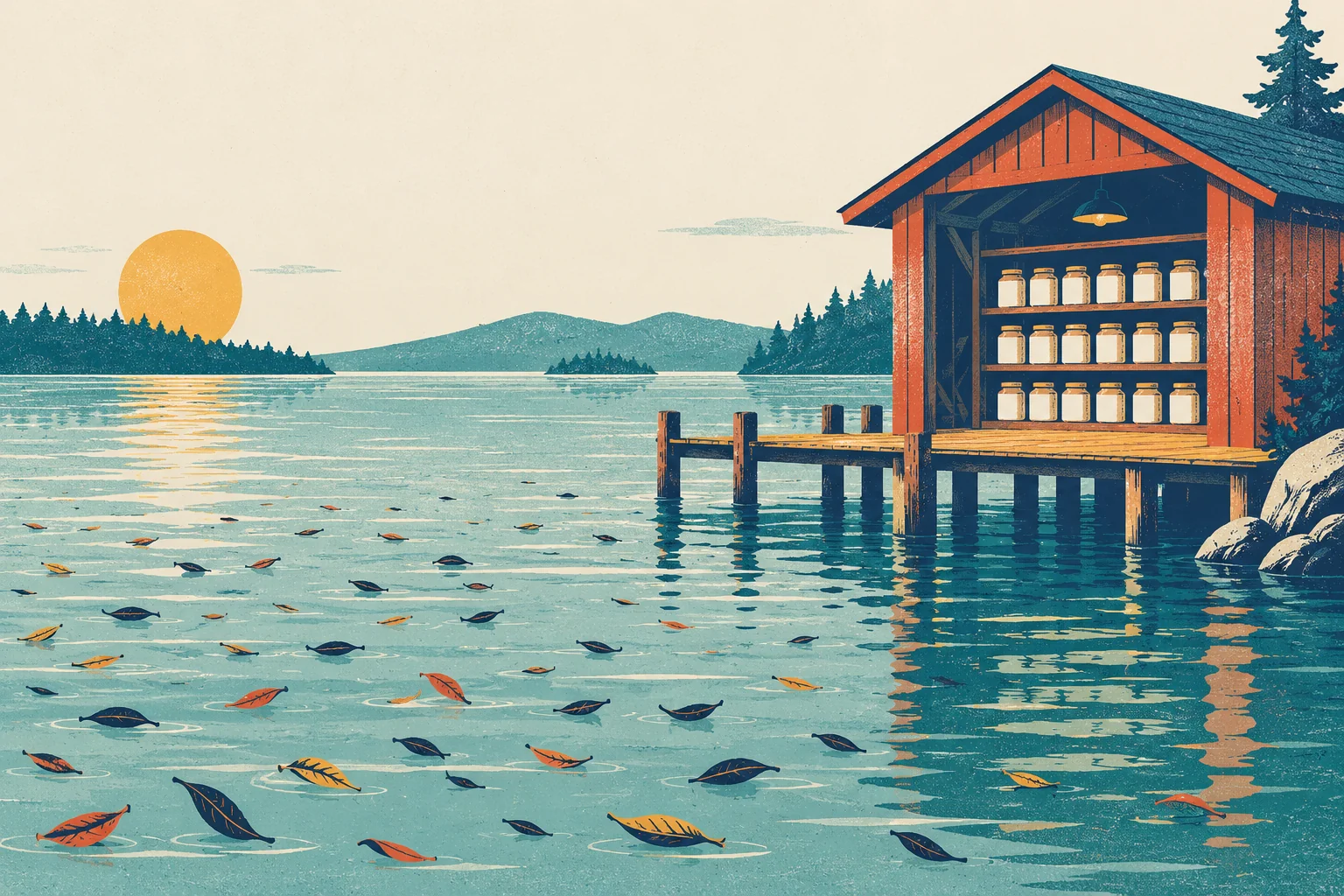
Look at the picture: a lake full of floating leaves, and a tidy boathouse with shelves of identical jars. The lake holds whatever falls into it. The boathouse holds only what someone has put on a shelf. And the boathouse does not stand on the shore. It stands on posts, in the lake. By the end of this chapter, you will see why.
The lake and the warehouse
In Chapters 9 and 10, you met Steep’s data lake: files kept in cheap storage, such as HDFS or object storage, in whatever format they arrived. A lake holds anything: tables in Parquet, events in JSON, logs, even images. Many engines can read the same files. Each reader applies a schema when it reads (schema-on-read). In the picture, the lake is the water, and the files are the leaves: many shapes, floating where they fell.
A data warehouse is the older idea. It is a database built for analysis. It stores its tables in its own managed format, checks every row against the schema when the row is written (schema-on-write), and lets many people query the same tables at once with SQL. It also controls who may read what. Companies such as Teradata have built warehouse systems for decades; today, cloud warehouses such as Snowflake, Google BigQuery and Amazon Redshift do the same job. In the picture, the warehouse is the boathouse: every jar on a shelf.
Data lake
Data warehouse
Stores
Files, in any format
Tables, in the warehouse’s own format
Schema
Applied when you read
Checked when you write
Cost of storage
Low
Higher
Changing one row
Hard (rewrite files)
Easy (UPDATE)
Who can read it
Many engines
Mostly the warehouse’s own engine
Main risk
Nobody knows what the files mean
Cost, and your data is locked inside
A word about names. Until now, this book has used “the warehouse” the way Steep’s staff do: for the whole data platform, the place where Steep collects and cleans its data (the Prologue’s definition). Strictly, Steep keeps that data as files in a lake: Parquet files in folders, described by Hive’s metastore (Chapters 9 and 10). On top of those files, it builds warehouse-style tables in layers, from raw copies to clean summaries (Chapter 12). So Steep’s “warehouse” is a set of plain Hive tables on a lake. A warehouse that stands on a lake has its own name, the lakehouse, and this chapter ends there.
A lake where nobody knows what the files mean, or which ones are current, is often called a data swamp. Steep’s lake was not a swamp. But it had a quieter weakness, and the chargeback found it.
Why a Hive table cannot take back a refund
Remember from Chapter 10: a file in HDFS is written once. Object storage works the same way: you can replace a whole file, but you cannot change a few bytes inside it. Parquet files are built to be written once too. So a plain Hive table cannot update a row (change it in place).
To record the chargeback, Steep’s nightly job must rewrite a whole partition: the folder dt=2026-08-19/city=harbor. In Hive’s SQL, that is INSERT OVERWRITE … PARTITION (…), which replaces everything in the folder. The job reads the whole folder, changes one row, and writes it all back: 2,533 rows, for one refund.
That one chargeback was not alone. From 15 September to the end of 25 September, 200 August orders were refunded, on every one of those eleven days. August has 124 folders in the lake (1 August to 31 August, four cities each). Each night, the job rewrites every folder that holds one of that day’s changes. Over those eleven nights, recording 200 changed rows means 171 folder rewrites and 324,247 rows written: about 1,621 rows written for each row that changed.
Rewriting is only the first problem. There are four more.
No safe moment to read. While the job replaces a folder’s files, a query that reads the folder can see some old files and some new ones, or none at all. Its answer can be wrong without any error.
No safe way to write twice. If two jobs rewrite the same folder at the same time, the last one wins, and the other one’s change is lost.
No memory. When a folder is overwritten, the old files are deleted. Nobody can ask what the table said last week. This is Mia’s question.
Slow planning. Hive’s metastore knows the table’s partitions, but not its files. To plan a query, an engine lists the files in every folder it needs. On object storage, listing thousands of folders takes time, and the small-files problem of Chapter 9 makes it worse.
Hive itself later added transactional tables that can update and delete rows. But they work only with ORC files, and other engines support them only in part. Most lakes kept their plain tables, with these problems.
A time machine made of the binlog
Mia did not need a new table to answer her question. MySQL had deleted most of its own August binlog files by now (after 30 days, as Chapter 7 explained). But she had Steep’s saved copy of the binlog, the lake table cdc_orders_binlog: every change to every order, in commit order. To see the orders table as it stood at the end of 14 September, replay every change up to that moment and stop. Then count August.
Table 1: August’s orders (placed 1–31 August), replayed from the binlog as of the end of three days.
As of
Completed orders
Net revenue
Refunded orders
End of 14 September (Dana’s question)
194,276
$2,419,745.03
1,679
End of 25 September (this chapter)
194,076
$2,417,213.40
1,879
End of the data, 25 October
193,976
$2,415,954.51
1,979
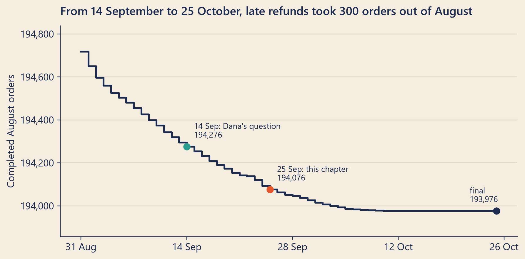
At the end of the day Dana asked her question, the database said August had 194,276 completed orders and $2,419,745.03 of net revenue. By the end of that Friday, 200 of those orders had been refunded, and August had lost $2,531.63. (The table counts whole days. At three o’clock that Friday, when Mia counted, 192 of these refunds had arrived; the other eight came that evening.)
This book’s data runs to 25 October, so we can look further ahead than Mia could. (The headline numbers in this book use final statuses; see Chapter 1.) The last August order changed on 10 October. In total, 300 August orders and $3,790.52 left August after 14 September. Each of these refunds arrived between 16 and 40 days after its order, 33 days in the middle. Of all of August’s 1,979 refunds up to 25 October, 1,237 had arrived by the time the month ended.
Show the code
after = asof[asof.as_of_date >= CLOSE_DAY]fig, ax = bk.figure(8, 3.9)ax.step(after.as_of_date, after.completed_orders, where="post", color=bk.INK, linewidth=2)marks = [(FIRST_REPORT, first, bk.TEAL, "14 Sep: Dana's question", (8, 10)), (STORY_DAY, story, bk.TOMATO, f"{STORY_DAY.day} Sep: this chapter", (8, 10)), (asof.as_of_date.iloc[-1], final, bk.INK, "final", (-30, 10))]for day, t, color, label, offset in marks: ax.plot([day], [t["completed_orders"]], "o", color=color, markersize=7, zorder=3) ax.annotate(f"{label}\n{bk.fmt_int(t['completed_orders'])}", (day, t["completed_orders"]), xytext=offset, textcoords="offset points", fontsize=9, color=bk.INK)ax.set_ylim(final["completed_orders"] -120, at_close.completed_orders +120)ax.yaxis.set_major_formatter(lambda v, _: f"{v:,.0f}")ax.xaxis.set_major_locator(mdates.WeekdayLocator(byweekday=mdates.MO, interval=2))ax.xaxis.set_major_formatter(lambda v, _: f"{mdates.num2date(v).day}{mdates.num2date(v):%b}")ax.set_ylabel("Completed August orders")ax.set_title(f"From 14 September to {day_month(world.END)}, late refunds took {bk.fmt_int(n_all)} orders out of August")plt.show()
Figure 1: August’s completed orders, as the database showed them at the end of each day after the month ended. The axis does not start at zero.
Replaying a binlog works, but it is slow and clumsy. To ask about one moment, you replay the history of every order. Theo had a better idea for the lake.
A table that keeps a diary
The idea behind modern lake tables fits on one napkin, and Theo drew it. On the left, a folder of Parquet files. On the right, a small notebook.
“Keep the files,” he said. “Never change them. But keep a list.”
Data files never change. New or changed rows go into new files. Old files stay as they are.
A list says which files make up the table. Next to the data files sits metadata: data about data. Its main job is to say which files form the table right now. Each version of that list is a snapshot: the table as it was after one change.
A change is a commit. To change the table, a writer first writes its new data files. Then it writes a new snapshot that lists the new set of files. Last, it makes the new snapshot the current one, in a single step. This last step is the commit. (Commit means “make final”. In Chapter 7, the database commits a piece of work; in Chapter 8, a reader commits its bookmark. Here, it is the moment a change becomes part of the table.) In Apache Iceberg, the commit changes one pointer: a small record that says which metadata file is the current one. A catalog, a small service, keeps these pointers for every table. In Delta Lake, the commit writes the next numbered file in the table’s log. If another writer committed first, the commit fails. The writer then checks the newer snapshot and tries again, or gives up if the two changes clash.
A reader starts from the current snapshot and reads exactly the files it lists. A change that is half written is not in any snapshot yet, so no reader can see it. This gives the table four promises, known by the letters ACID:
Atomic: a change happens completely, or not at all.
Consistent: every commit takes the table from one valid state to another.
Isolated: readers and writers working at the same time do not see each other’s half-done work.
Durable: once a change is committed, it stays.
The snapshots also give three gifts.
Time travel. Old snapshots stay until someone deletes them. So you can ask for the table as it was at an earlier moment. In Spark SQL, on an Iceberg or Delta Lake table:
SELECTcount(*) AS completed_orders, sum(net_amount) AS net_revenueFROM ods_orders TIMESTAMPASOF'2026-09-14 23:59:59'WHERE dt BETWEEN'2026-08-01'AND'2026-08-31'AND status ='completed';
Is that Mia’s question in one query? Only if the table was kept up to date. If CDC changes were merged into ods_orders every few minutes, this query would return almost the same answer as the replay. But Steep loads once a night, at 2 a.m. (Chapter 13). The last load before 23:59 on 14 September held changes up to the end of 13 September. One more detail: the engine reads the time in the query in the time zone of your connection, so set it to Steep’s.
Schema evolution. A schema can change over time: a new column, a renamed column, a wider number type. The metadata records each change, so old files need not be rewritten. Iceberg gives every column a permanent ID, so renaming a column never mixes up its data with another column’s.
Merge. A table format can update rows, so it can apply a stream of changes directly. The SQL statement MERGE matches incoming rows to existing rows by a key. It updates the rows that match and inserts the rows that do not. Doing both at once is called an upsert (update or insert). Teams often apply CDC changes to a lake table this way, every few minutes:
MERGEINTO ods_orders AS tUSING order_changes AS s -- the newest change per order, from the binlogON t.order_id = s.order_idWHEN MATCHED AND s.op ='d'THENDELETEWHEN MATCHED THENUPDATESET status = s.status, updated_at = s.updated_atWHENNOT MATCHED AND s.op <>'d'THENINSERT (order_id, status, net_amount, updated_at)VALUES (s.order_id, s.status, s.net_amount, s.updated_at);
(The real table has more columns. This sketch shows the shape.)
How does a table format change one row, if files never change? There are two ways.
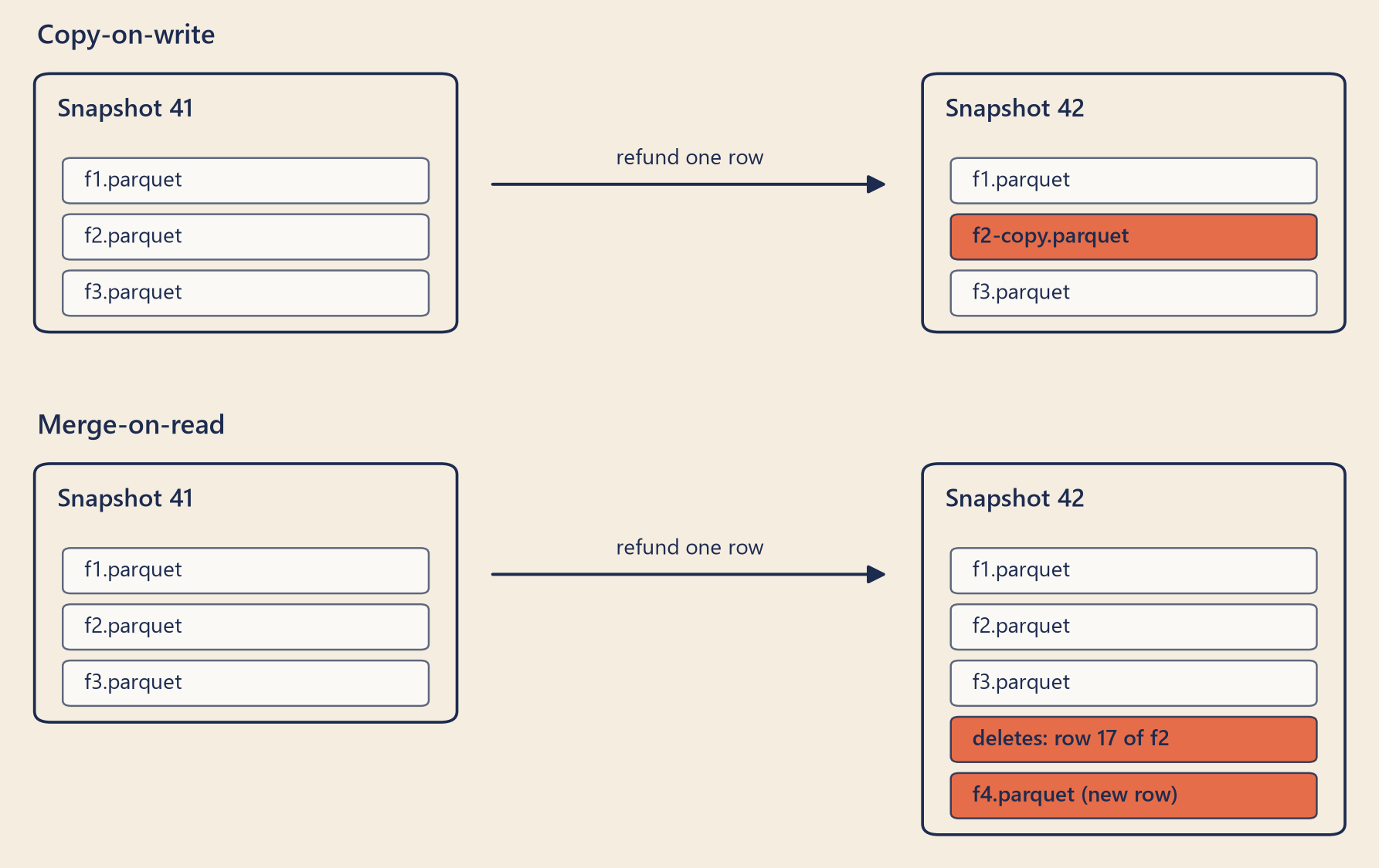
Copy-on-write. Rewrite each data file that holds a changed row. The new snapshot lists the new copy instead of the old file. Writing costs more. Reading stays fast, because readers see plain files. This is the same idea as Hive’s rewrite, but per file, not per folder, and with a commit and a snapshot.
Merge-on-read. Leave the old file alone. Write a small file that says which rows are deleted, plus a new file with the new versions. Readers merge them while they read. Writing is cheap. Reading costs more, until a compaction job merges the small files back into big ones.
Show the code
bk.setup()fig, ax = plt.subplots(figsize=(8, 5.0), layout="constrained")ax.set_axis_off()ax.set_xlim(-0.15, 9.85)ax.set_ylim(-0.45, 8.75)def snapshot(x, y, title, files):"""A snapshot box listing its files; new files in tomato.""" h =0.62*len(files) +0.95 ax.add_patch(FancyBboxPatch((x, y - h), 3.1, h, boxstyle="round,pad=0.02,rounding_size=0.12", facecolor=bk.PAPER, edgecolor=bk.INK, linewidth=1.2)) ax.text(x +0.15, y -0.38, title, fontsize=10.5, fontweight="semibold", color=bk.INK, va="center")for i, (name, new) inenumerate(files): fy = y -0.95-0.62* i ax.add_patch(FancyBboxPatch((x +0.2, fy -0.45), 2.7, 0.48, boxstyle="round,pad=0.01,rounding_size=0.06", facecolor=bk.TOMATO if new else"#ffffff", alpha=0.85if new else0.7, edgecolor=bk.INK, linewidth=0.8)) ax.text(x +0.35, fy -0.21, name, fontsize=9, color=bk.INK, va="center", fontweight="semibold"if new else"normal")def arrow(y): ax.add_patch(FancyArrowPatch((3.35, y), (6.35, y), arrowstyle="-|>", mutation_scale=16, color=bk.INK, linewidth=1.3)) ax.text(4.85, y +0.22, "refund one row", fontsize=9, color=bk.INK, ha="center")base = [("f1.parquet", False), ("f2.parquet", False), ("f3.parquet", False)]ax.text(0, 8.45, "Copy-on-write", fontsize=11.5, fontweight="semibold", color=bk.INK)snapshot(0, 8.1, "Snapshot 41", base)arrow(6.9)snapshot(6.6, 8.1, "Snapshot 42", [("f1.parquet", False), ("f2-copy.parquet", True), ("f3.parquet", False)])ax.text(0, 4.15, "Merge-on-read", fontsize=11.5, fontweight="semibold", color=bk.INK)snapshot(0, 3.8, "Snapshot 41", base)arrow(2.6)snapshot(6.6, 3.8, "Snapshot 42", base + [("deletes: row 17 of f2", True), ("f4.parquet (new row)", True)])plt.show()
Figure 2: One refund in a table format. Each box is a snapshot: the list of files that make up the table. Old files stay on disk, so the old snapshot can still be read (time travel).
Time travel has a limit. Old snapshots keep old files on disk, and disk costs money. So teams delete old snapshots and their files on a schedule, and the time travel to those moments goes with them. (The box “Under the hood” gives the details for Iceberg and Delta Lake.)
Four table formats
A table format is this set of rules: how data files, metadata and snapshots are laid out and committed. It sits on top of a file format such as Parquet. Four open table formats are common today. All four give ACID commits, snapshots and time travel. They differ in where they put their effort.
Format
Started at
Best known for
Apache Iceberg
Netflix
Planning from metadata; safe schema changes
Delta Lake
Databricks
A simple log of numbered commits; close to Spark
Apache Hudi
Uber
Fast updates by record key; incremental queries
Apache Paimon
Apache Flink (as Flink Table Store)
Streaming updates from Flink
Iceberg keeps its metadata as a tree of files, so a query can find its data files without listing any folders. With hidden partitioning, the table works out partition values itself, such as the day of a timestamp.
Delta Lake keeps its history in a folder called _delta_log, with one numbered file per commit. It works most closely with Spark.
Hudi gives every record a record key and keeps an index to find it fast. It also answers incremental queries: “only the rows that changed since this moment.”
Paimon was built for streaming writes from Flink. It keeps tables with a key in an LSM tree (log-structured merge tree), which takes many small updates quickly and merges them later.
The lakehouse
Now look at the picture once more. The boathouse does not have its own water. It stands on posts in the lake. But inside, everything has a shelf and a place.
A lakehouse is that idea for data: lake storage, with warehouse behaviour on top. The files stay cheap and open, in object storage. A table format adds transactions, schemas, snapshots and time travel. A catalog adds names and permissions. Then the same copy of the data serves dashboards, SQL analysts, and machine learning, with no need to copy everything into a separate warehouse first.
The jars in the boathouse are still blank. Choosing what goes on each shelf, and how to label it, is the work of the next chapter.
Engines that read the lake
A table format is only a set of rules for files. To ask a question, you still need a query engine: a program that reads the files, runs the SQL, and returns the answer. Because the formats are open, one table can serve many engines. Spark (Chapter 10) and Flink (Chapter 14) read and write them. Three other names come up often.
Engine
What it is
Keeps its own data?
Trino
A distributed SQL engine
No: it reads data where it lives
ClickHouse
A column-oriented database for fast analysis
Yes, and it can read lake tables
Apache Doris, StarRocks
MPP databases that speak MySQL’s protocol
Yes, and they can read lake tables
Trino stores no data. Through connectors, one query can join a lake table with a table in a database such as MySQL.
ClickHouse keeps its own tables in its MergeTree storage engines. It can also read Iceberg and Delta Lake tables in place.
Apache Doris and StarRocks are MPP databases: massively parallel processing, where many machines each work on their share of one query. Both are popular for fast dashboards on fresh data. Both can read Hive tables and the main table formats.
NoteUnder the hood
A table as a list of files. Write \(F_v\) for the set of data files in snapshot \(v\), and \(D_v\) for the rows that its delete files remove. The table at snapshot \(v\) is every row in the files of \(F_v\), minus the rows in \(D_v\). A commit reads snapshot \(v\), writes new files, and proposes \(F_{v+1} = (F_v \setminus \text{removed}) \cup \text{added}\). It succeeds only if \(v\) is still the current snapshot. This is optimistic concurrency: assume no conflict, check at the end, and retry if someone else committed first.
Time travel, precisely. “As of time \(t\)” means the newest snapshot whose commit time is at or before \(t\). The commit time is when the change reached the table, not when the event happened in the world. Our replay of the binlog follows the same idea: it applies the changes in binlog order, which is commit order, and stops at a time. (Strictly, a binlog entry’s timestamp is when its statement started, a moment before the commit.) So “August as of 14 September” answers what did the table say then?, not what was true then? A chargeback on 25 September makes an August order refunded from 25 September on, in every “as of” view.
Iceberg’s metadata tree. Table metadata file (schema, partition spec, list of snapshots, current snapshot) → one manifest list per snapshot → manifest files (one entry per data file, with its partition values and column statistics) → data files. A commit writes a new metadata file and asks the catalog to swap its pointer from the old file to the new one. Format version 2 added delete files; version 3 added deletion vectors. Snapshots are expired by a maintenance procedure, which by default removes snapshots older than five days; it does not run by itself.
Delta Lake’s log._delta_log/00000000000000000000.json, …01.json, and so on, zero-padded to 20 digits. Each file lists actions such as add file and remove file. Parquet checkpoint files summarise the log so far. VACUUM deletes data files that the current version no longer uses and that are older than the retention period (7 days by default), even if an older version still needs them; log entries are kept for 30 days by default (delta.logRetentionDuration). Time travel needs both the log and the data files.
Hudi’s two table types. Copy On Write: updates write new versions of the base files. Merge On Read: updates go to log files (often Avro, a row format) beside the base files; queries merge them, and compaction folds them into new base files.
Copy-on-write or merge-on-read, and cleaning up. Iceberg lets each table choose copy-on-write or merge-on-read for deletes, updates and merges; its default is copy-on-write. Delta Lake’s deletion vectors and Iceberg’s format version 3 mark deleted rows without rewriting the file, which is merge-on-read. Iceberg’s expiring snapshots removes old snapshots and the files that only they used; after that, time travel to them is gone.
Hive’s transactional tables.UPDATE and DELETE arrived in Hive 0.14 and MERGE in Hive 2.2. The table must be stored as ORC and marked transactional=true.
Who looks after the formats. Iceberg became a top-level Apache project in 2020, and Paimon in 2024; Delta Lake is hosted by the Linux Foundation. Hudi records every action on a table in its timeline. Paimon can also produce a complete changelog for streaming readers, if a table is set up for it.
The engines. Trino was called PrestoSQL until December 2020. ClickHouse reads lake tables with table functions such as iceberg() and deltaLake(). Doris began at Baidu; StarRocks grew from the Doris code and is a Linux Foundation project. Both reach lake tables through external catalogs: Doris for Hive, Iceberg, Hudi and Paimon (Delta Lake is experimental), StarRocks for all five.
Paimon’s LSM tree. Each bucket of a primary-key table keeps sorted runs of rows. New writes form small runs, and background compaction merges runs. When two rows have the same key, a merge engine decides the result: keep the latest (the default), fill in only the columns that changed (partial update), or add them up (aggregation).
Try it
The time machine. Move the slider to choose an “as of” day. The page shows August as the database showed it at the end of that day, and lists the August orders that changed after 14 September, up to that day.
ttDb = {try {returnawait DuckDBClient.of({august_as_of:FileAttachment("../data/out/web/cdc_august_as_of.parquet"),binlog:FileAttachment("../data/out/web/cdc_orders_binlog_sample.parquet") }); } catch (error) {returnnull;// the readout below explains what went wrong }}
Show the code
ttData = {if (ttDb ===null) returnnull;const h = ttFacts.hoursBehindUtc;const series =await ttDb.query(` SELECT strftime(as_of_date, '%Y-%m-%d') AS day, completed_orders::DOUBLE AS orders, net_revenue::DOUBLE AS revenue, refunded_orders::DOUBLE AS refunded FROM august_as_of WHERE as_of_date >= DATE '${ttFacts.first}' ORDER BY as_of_date`);const changes =await ttDb.query(` WITH placed AS ( SELECT order_id, CAST(ts - INTERVAL ${h} HOUR AS DATE) AS placed_on FROM binlog WHERE op = 'c' ), refunds AS ( SELECT order_id, ts, before.net_amount::DOUBLE AS amount FROM binlog WHERE op = 'u' AND after.status = 'refunded' ) SELECT r.order_id, strftime(p.placed_on, '%Y-%m-%d') AS placed_on, strftime(r.ts - INTERVAL ${h} HOUR, '%Y-%m-%d') AS refunded_on, r.amount FROM refunds AS r JOIN placed AS p ON p.order_id = r.order_id WHERE p.placed_on BETWEEN DATE '2026-08-01' AND DATE '2026-08-31' AND CAST(r.ts - INTERVAL ${h} HOUR AS DATE) > DATE '${ttFacts.firstReport}' ORDER BY r.ts`);const asRows = rows =>Array.from(rows, r => (typeof r.toJSON==="function"? r.toJSON() : r));return {series:asRows(series).map(r => ({day: r.day,orders:Number(r.orders),revenue:Number(r.revenue),refunded:Number(r.refunded)})),changes:asRows(changes).map(r => ({id:String(r.order_id),placed: r.placed_on,refunded: r.refunded_on,amount:Number(r.amount)})) };}
Show the code
viewof ttIndex = Inputs.range([0, ttData ===null?1: ttData.series.length-1], {step:1,label:"Days after August ended",value: ttData ===null?0:Math.max(0, ttData.series.findIndex(d => d.day=== ttFacts.storyDay))})
Show the code
{const C = {teal:"#2a9d8f",tealText:"#1f7a6f",tomato:"#e4572e",tomatoText:"#b8401c",mustard:"#f2b134",ink:"#1d2b4f",muted:"#8a8f9e",grid:"#d9cfbd",deep:"#ebe2d0"};const wrapStyle ="font-family:Inter,system-ui,sans-serif;color:"+ C.ink;if (ttData ===null|| ttData.series.length===0) {return htl.html`<p style="${wrapStyle};font-size:0.85rem">The data files could not be loaded in this browser.</p>`; }const S = ttData.series;const i =Math.min(ttIndex, S.length-1);const cur = S[i];const ref = S.find(d => d.day=== ttFacts.firstReport);const fmt = x =>Math.round(x).toLocaleString("en-US");const usd = x =>"$"+ x.toLocaleString("en-US", {minimumFractionDigits:2,maximumFractionDigits:2});const MONTHS = ["January","February","March","April","May","June","July","August","September","October","November","December"];const parts = d => d.split("-").map(Number);const nice = d => { const [, m, dd] =parts(d);return`${dd}${MONTHS[m -1]}`; };const short = d => { const [, m, dd] =parts(d);return`${dd}${MONTHS[m -1].slice(0,3)}`; };// no break inside a date// --- the chart: August's completed orders as of each day ---const W =Math.max(300,Math.min(660, width)), H =210;const L =62, R =14, T =16, B =30;const ys = S.map(d => d.orders);const lo =Math.min(...ys) -60, hi =Math.max(...ys) +60;const x = k => L + (W - L - R) * k / (S.length-1);const y = v => T + (H - T - B) * (hi - v) / (hi - lo);let path =`M${x(0)},${y(S[0].orders)}`;for (let k =1; k < S.length; k++) path +=`H${x(k)}V${y(S[k].orders)}`;const k14 = S.findIndex(d => d.day=== ttFacts.firstReport);const ticks = [0, S.length-1];const svg = htl.svg`<svg viewBox="0 0 ${W}${H}" width="${W}" height="${H}" role="img" aria-label="August's completed orders as of each day; the selected day is ${nice(cur.day)}" style="max-width:100%;font-family:Inter,system-ui,sans-serif">${[lo +60, hi -60].map(v => htl.svg`<line x1="${L}" x2="${W - R}" y1="${y(v)}" y2="${y(v)}" stroke="${C.grid}"/> <text x="${L -6}" y="${y(v) +4}" text-anchor="end" font-size="11" fill="${C.ink}">${fmt(v)}</text>`)} <line x1="${x(k14)}" x2="${x(k14)}" y1="${T}" y2="${H - B}" stroke="${C.teal}" stroke-dasharray="4 3"/> <text x="${x(k14) +5}" y="${T +10}" font-size="11" fill="${C.tealText}">14 Sep</text> <path d="${path}" fill="none" stroke="${C.ink}" stroke-width="2"/> <circle cx="${x(i)}" cy="${y(cur.orders)}" r="6" fill="${C.tomato}" stroke="${C.ink}"/>${ticks.map(k => htl.svg`<text x="${x(k)}" y="${H -10}" text-anchor="${k ===0?"start": k === S.length-1?"end":"middle"}" font-size="11" fill="${C.ink}">${short(S[k].day)}</text>`)} </svg>`;// --- the readout ---const dOrders = cur.orders- ref.orders, dRevenue = cur.revenue- ref.revenue;const signed = (v, f) => (v >0?"+": v <0?"−":"±") +f(Math.abs(v));const before14 = cur.day< ttFacts.firstReport;const shown = ttData.changes.filter(c => c.refunded<= cur.day);const listSum = shown.reduce((s, c) => s + c.amount,0);const matches =!before14 && shown.length===-dOrders &&Math.abs(listSum + dRevenue) <0.005;const sql =`-- In a table format (Spark SQL on Iceberg or Delta Lake).-- With a nightly load, this shows the table as of the-- last load before this moment, not a full replay.SELECT count(*) AS completed_orders, sum(net_amount) AS net_revenueFROM ods_orders TIMESTAMP AS OF '${cur.day} 23:59:59'WHERE dt BETWEEN '2026-08-01' AND '2026-08-31' AND status = 'completed';`;const sqlBox = htl.html`<pre class="tt-sql"><code></code></pre>`; sqlBox.querySelector("code").textContent= sql;const recent = shown.slice(-6).reverse();const style = htl.html`<style> .tt-wrap { font-family: Inter, system-ui, sans-serif; color: ${C.ink}; } .tt-day { font-size: 1.05rem; margin: 0.3rem 0 0.5rem; } .tt-cards { display: flex; flex-wrap: wrap; gap: 0.5rem; margin-bottom: 0.6rem; } .tt-card { flex: 1 1 9rem; border: 1px solid rgba(29,43,79,0.18); border-radius: 6px; padding: 0.4rem 0.6rem; background: rgba(255,255,255,0.55); } .tt-card .k { font-size: 0.75rem; color: #3d4766; } .tt-card .v { font-size: 1.1rem; font-weight: 600; font-variant-numeric: tabular-nums; } .tt-card .d { font-size: 0.78rem; color: ${C.tomatoText}; font-variant-numeric: tabular-nums; } .tt-note { font-size: 0.84rem; color: #3d4766; } .tt-list { width: 100%; border-collapse: collapse; font-size: 0.74rem; font-variant-numeric: tabular-nums; } .tt-wrap table.tt-list { display: table; } .tt-list th, .tt-list td { padding: 0.2rem 0.25rem; border-bottom: 1px solid rgba(29,43,79,0.12); text-align: left; } .tt-list td:first-child, .tt-list td.num { white-space: nowrap; } .tt-list td.num { text-align: right; } .tt-sql, .tt-sql code { font-size: 0.74rem; line-height: 1.4; white-space: pre-wrap; overflow-wrap: anywhere; } .tt-sql { background: ${C.deep}; padding: 0.6rem 0.8rem; border-radius: 6px; } </style>`;return htl.html`<div class="tt-wrap">${style} <p class="tt-day" aria-live="polite">August, as the database showed it at the end of <strong>${nice(cur.day)}</strong>:</p> <div class="tt-cards"> <div class="tt-card"><div class="k">Completed orders</div><div class="v">${fmt(cur.orders)}</div> <div class="d">${signed(dOrders, fmt)} vs 14 Sep</div></div> <div class="tt-card"><div class="k">Net revenue</div><div class="v">${usd(cur.revenue)}</div> <div class="d">${signed(dRevenue, usd)} vs 14 Sep</div></div> <div class="tt-card"><div class="k">Refunded so far</div><div class="v">${fmt(cur.refunded)}</div></div> </div>${svg} <p class="tt-note">The dashed teal line is 14 September, the day of Dana's question. The tomato dot is your "as of" day.</p>${before14 || cur.day=== ttFacts.firstReport? htl.html`<p class="tt-note">${before14 ?"This day is before 14 September.":"This is 14 September itself, the reference day."} Move the slider to a later day to list the orders that changed after Dana's question.</p>`: htl.html`<p class="tt-note"><strong>${shown.length}</strong> August orders were refunded after 14 September and up to this day, for ${usd(listSum)}. ${matches ?"That matches the change in the totals above, to the cent.":""}${recent.length?"The newest ones:":""}</p>${recent.length? htl.html`<table class="tt-list"><thead><tr><th>Order</th><th>Placed → refunded</th><th class="num">$</th></tr></thead> <tbody>${recent.map(c => htl.html`<tr><td>${c.id}</td><td>${short(c.placed)} → ${short(c.refunded)}</td> <td class="num">${c.amount.toFixed(2)}</td></tr>`)}</tbody></table>`:""}`} <p class="tt-note">The same question, asked of a table format with time travel. It matches the replay only if changes were merged into the table soon after they happened:</p>${sqlBox} </div>`;}
Things to try:
Start at 25 September, the day of this chapter. Then move the slider back to 14 September: the change is zero, because that is the reference day.
Move to the right end. After 10 October, August stops changing.
Move to the left end, 31 August, the day August ended. Even then, refunds still had weeks to arrive.
The totals were replayed in advance from the full binlog, one row per day. The list of orders comes from the binlog itself, live in your browser. The two are separate calculations, and they agree.
Common traps
Comparing numbers with different “as of” times. August on 14 September and August today are two different numbers, and both are honest. Write the “as of” time next to every number you report.
Treating time travel as a backup. Snapshots live in the same storage as the table, and they are deleted on a schedule. A backup is a separate copy, kept somewhere else.
Reading “as of” as “what was true”. Time travel shows what the table said at a commit time. A late refund changes the past only from the day it arrives.
Committing too often. A stream that commits every few seconds creates many small files and many snapshots. Schedule compaction and snapshot expiry.
Two catalogs for one table. If two engines register the same files in two catalogs, each sees its own current snapshot. Choose one catalog as the source of truth.
TipAudit Instinct · As originally reported, and as restated
Accountants close a month. When a refund for an August sale arrives in September, it is normally booked in September. August’s ledger does not move. Only an error in August’s figures leads to a restatement: August is shown again, corrected, next to the figure as originally reported, with a note that explains the difference.
Steep’s orders table follows a different rule. It counts orders by the day they were placed, with their status today. So its August keeps moving for weeks. Neither rule is wrong, but a report must say which one it uses. Dana’s board will see August twice: in finance’s closed books, and in the warehouse. The two will differ, because one books each refund on the day it arrives and the other on the day of its order. With the binlog, Mia can explain the difference refund by refund.
Cut-off testing compares when a transaction really happened with the period in which it was recorded. Snapshots and binlog positions give the second date: they show what the table said, and when.
NoteInterview Corner
Q1. Why did teams move from plain Hive tables to Iceberg, Hudi or Delta Lake?
NoteA short answer
Plain Hive tables track only partitions. Changing a row means rewriting its partition, readers can see a rewrite half done, two writers can overwrite each other, and nothing records the old version. Planning a query means listing folders, which is slow on object storage. Table formats track every file in snapshot metadata. That gives ACID commits, row-level UPDATE, DELETE and MERGE (copy-on-write rewrites only the affected files; merge-on-read writes small delete or log files and merges them at read time), time travel and rollback, schema and partition evolution without rewriting data, file-level statistics for skipping, and built-in compaction. The formats are open, so many engines can share one table.
Q2. What is time travel useful for?
NoteA short answer
Reproducing a report exactly as it was first published, for an audit or a dispute. Debugging: compare today’s snapshot with yesterday’s to see what changed. Rolling back a bad write by making an older snapshot current again. Keeping a machine-learning training set reproducible. Its limits: it reaches back only as far as snapshots are kept, it follows commit time rather than business time, and it is not a backup.
Q3. Data lake, data warehouse, lakehouse: what is the difference?
NoteA short answer
A lake stores files of any kind in cheap storage, applies the schema when reading, and lets many engines share the data, but on its own it has no transactions and weak control over what the files mean. A warehouse stores managed tables, checks the schema on write, supports transactions and fast SQL, and governs access, but it costs more and keeps the data in its own format. A lakehouse puts a table format and a catalog on top of lake storage, so open files behave like warehouse tables: one copy of the data for dashboards and reports (business intelligence, or BI), SQL and machine learning.
That afternoon, Mia went back to her own numbers. If August had moved, the two weeks of the case had moved too. She replayed the binlog to the start of 14 September, the same moment as finance’s spreadsheet in Chapter 1, and counted the completed orders of those two weeks.
The week before: 45,627. The week of the drop: 43,494. A fall of 4.7%. Then she replayed to that afternoon: a fall of 4.9%. The week of the drop was newer, so fewer of its refunds had arrived yet. That is why the fall looked a little smaller at first.
“So the refunds moved your number,” said Theo.
“By a fraction of a point,” said Mia. “And they cannot touch Dana’s dashboard at all. It counts the app’s payment events. A refund does not delete an event.” She wrote the two numbers in her notebook, each with its date.
This book can look past that Friday. With every refund in, by 25 October, the end of the data, the fall is 5.0%: the final-status number this book has used since Chapter 1.
Reported change: −12.0% orders, the week of 7 September compared with the week before (CEO dashboard).
Explained so far: 0 of the 12 points. About 7 of them sit between the orders database and the dashboard (Clue 1).
Suspects: the app, and the service that writes to Kafka (Chapter 8). The iOS app, version 3.2.0, is the main suspect (Chapter 6). Not proved.
Ruled out: the matcha menu (Chapter 4), Kafka (Chapter 8), storage (Chapter 9), computing (Chapter 10), and now refunds and restatements. Late refunds take completed orders out of finance’s count, more of them from the newer week. So finance’s fall grows, from 4.7% at the start of 14 September to 4.9% that Friday afternoon, closer to the dashboard’s −12.0%. The gap between finance’s count and the dashboard shrinks: from 7.3 to 7.1 points. The dashboard counts payment events, which refunds never remove. (By 25 October, the end of the data, that gap is 7.0 points: refunds moved it by less than half a point. They cannot explain 7.)
Open questions: Which orders have no order_completed event, and why? Did iOS 3.2.1, released on 24 September, fix it? (Chapter 15.)
New evidence: 192 August orders were refunded between 14 September and that Friday afternoon. A table that remembers can answer “as of when?” for any number. New rule: every number gets an “as of”.
Recap
A data lake keeps cheap, open files of any kind; a data warehouse keeps managed tables with transactions. Plain Hive tables on a lake cannot update a row, cannot commit safely, and forget every old version.
Table formats (Iceberg, Delta Lake, Hudi, Paimon) keep data files unchanged and add a log of snapshots. That gives ACID commits, MERGE, schema evolution and time travel. Lake storage with this warehouse behaviour is a lakehouse.
Data changes after the fact: by 25 October, the end of the data, 300 August orders had been refunded after 14 September. Every number needs an “as of” time, and a table that remembers can reproduce it.
English
中文
data lake
数据湖
data warehouse
数据仓库
lakehouse
湖仓一体
data swamp
数据沼泽
chargeback
拒付 / 退单
table format
表格式
metadata
元数据
snapshot
快照
commit
提交
catalog
目录
ACID
事务特性(原子性、一致性、隔离性、持久性)
time travel
时间旅行
schema evolution
模式演进
upsert / merge
更新插入 / 合并
copy-on-write
写时复制
merge-on-read
读时合并
compaction
合并 / 压实
deletion vector
删除向量
query engine
查询引擎
MPP (massively parallel processing)
大规模并行处理
restatement
重述
as originally reported
原报告数
cut-off testing
截止性测试
Further reading
Michael Armbrust and others, “Delta Lake: High-Performance ACID Table Storage over Cloud Object Stores”, Proceedings of the VLDB Endowment 13(12), 2020, pages 3411–3424. doi:10.14778/3415478.3415560. How a log of commits turns files in object storage into ACID tables.