10 · Too Big for One Machine: HDFS, Hive, and Spark
At six o’clock on Thursday morning, Steep released version 3.2.1 of its iOS app. The release note said only: Bug fixes and improvements.
Mia wrote the date and the time in her notebook. A fix is a claim, she thought. Claims need tests. She would test this one later.
Then she went back to the question that had slowed down checkout the day before. Was the gap new, or had something like it happened earlier in the summer? Her small charts had shown the gap in every city (Chapter 5), but they started in August. This time she would ask the lake, not production.
Her plan was clear. For every checkout_start event since 1 June, find the same user’s next event. If the payment worked, the next event should be order_completed. Then count, week by week and city by city, how often it was.
Her notebook had a second word for the day: computing. The dashboard’s numbers come out of jobs like hers, run on the same machines. Kafka was cleared, and so was the lake. But if the jobs after the lake lost events, part of the gap would belong to them, not to the app side.
The lake held 6.7 million cleaned app events since 1 June. That is the copy of Steep’s data that comes with this book: a sample small enough for a laptop. In the story, Steep’s real event history is far larger, with billions of rows. Too big for one machine. So Theo sent her query to Steep’s Spark cluster: a group of computers that share the work of one query. (You will meet Spark properly below.)
Mia’s query split the events by city, because she wanted one answer per city. At eleven, Theo opened the job’s status page. Steep’s cluster had eight machines. One step of the job had 200 small pieces of work, and Spark handed them out to the eight machines. (Steep’s cluster still ran with adaptive execution turned off. You will see below why that matters.) Of these, 196 had finished in less than a second. Three had finished in a few minutes. One was still running.
“Which one is that?” asked Mia.
“Harbor,” said Theo. The Harbor piece ran until the middle of the afternoon.
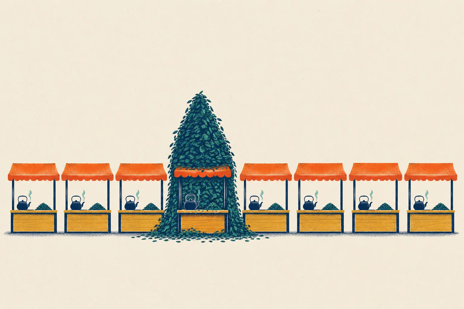
He took a napkin and drew a row of eight tea stalls, one for each machine. Three had a small pile of leaves. Four had none at all. On the last one he drew a mountain.
“You split the work by city,” he said. “Steep has four cities, so only four machines got any work. The other machines had nothing to do. And Harbor is our biggest city: since June, 40% of all the events. One machine got all of them. The job could not finish until that one machine did.”
“In audit,” said Mia, “we call that an engagement held up by one big subsidiary.”
“Same problem, same fix,” said Theo. “Let me show you how the machines share work. Then we fix your query.”
Mia wrote: Not too big. Badly split.
ImportantThe big idea
Split the work across many machines, and make sure no single machine gets most of it.
Look at the picture: eight stalls, seven nearly finished with their small piles, and one buried under a mountain, its kettle still cold. The market closes only when the last stall is done. (Theo’s napkin was worse: in Mia’s job, four of the stalls got no leaves at all.)
Why one machine is not enough
Suppose you must read 10 terabytes (ten million megabytes) from one disk. Say the disk reads 200 MB per second. Reading alone then takes 50,000 seconds: about 14 hours, before any real work starts. (These are round numbers, for illustration.)
There are two ways out. You can buy a bigger machine: this is scaling up. It works until the biggest machine is not big enough, or costs too much. Or you can use many ordinary machines together: this is scaling out. A group of machines that work together is a cluster, and each machine in it is a node. A job that runs on many nodes at once is distributed.
Scaling out raises two questions. Where does the data live? And which machine does which part of the work? In the 2000s, the open-source project Apache Hadoop answered both, with ideas that Google had published in 2003 and 2004. The answer to the first question was HDFS. The answer to the second was MapReduce.
Splitting the data: HDFS
HDFS, the Hadoop Distributed File System, makes many machines look like one very large disk. It rests on four ideas.
Blocks. HDFS cuts every file into blocks: 128 MB each by default. Every block of a file has the same size, except the last one, which holds what is left. A 1 GB file becomes 8 blocks, and the blocks can live on different machines.
Copies. HDFS stores each block on several machines: 3 by default. This number is the replication factor, as for Kafka (Chapter 8). If one machine dies, two copies remain, and HDFS makes a new third copy elsewhere.
One map, many stores. One server, the NameNode, keeps the map of the file system: which files exist, which blocks belong to each file, and which machines hold each block. It keeps this map in memory. The other servers, the DataNodes, store the blocks. They report to the NameNode with regular “I am alive” messages, called heartbeats.
Write once. A file in HDFS is written once and then read many times. You can add to its end, but you cannot change bytes in its middle. (Remember this. It matters in Chapter 11.)
There is one more trick. Moving a program is cheaper than moving terabytes of data. So a distributed job tries to run each piece of work on a machine that already holds the block it needs. This is data locality.
What would Steep’s events look like in HDFS? The lake keeps one file per day: 115 files since 1 June, 2.7 MB each on average. Every one of them is far smaller than one block. So HDFS would keep 115 blocks, each three times: 345 block copies. If the same bytes were in one big file, they would need three blocks. A small file does not fill a whole block on disk. Its real cost is a record in the NameNode’s memory. This is the small-files problem of Chapter 9, seen from HDFS’s side: the NameNode must remember every file and every block.
Today, many teams keep their lake in object storage instead, such as Amazon S3 or Alibaba Cloud OSS. You store and fetch whole files, called objects, over the network, and the cloud company keeps the copies. Storage and computing are separate: a cluster can start, read the files, and shut down when it is done. The ideas in this chapter still apply. Only the place where the files live has changed.
Giving files a table: Hive
Files in folders are not yet a table. To ask a SQL question, an engine must know which files belong to the table, which columns they hold, and how to read them. Apache Hive added this to Hadoop. It was built at Facebook and described in 2009.
Hive keeps that knowledge in the metastore: a small, ordinary database that holds a description of every table. For each table, it stores the columns and their types, the file format, the folder where the files live (the table’s location), and the list of its partitions. The metastore holds no rows of data, only the description. Several engines can share one metastore: Hive, Spark and Trino (another SQL engine for files) can all read it. So a table defined once can be queried from all of them.
Here is how Steep could define its events table in Hive’s SQL:
CREATE EXTERNAL TABLE ods_events ( event_id STRING, event_name STRING, user_id STRING, order_id BIGINT, event_time TIMESTAMP-- ... and the other columns)PARTITIONED BY (dt STRING)STORED AS PARQUETLOCATION '/lake/ods/ods_events';
Three ideas sit in these few lines.
Schema-on-read. A schema is the list of a table’s columns and their types (Chapter 9). A traditional database checks every row against the schema when the row is written, and it refuses a row that does not fit. This is schema-on-write. Hive checks nothing when files arrive. The files are placed in the table’s folder as they are, and Hive applies the schema only when it reads them. This is schema-on-read. Loading is fast and flexible. The price is that a bad file is found only when someone reads it. In a text file, a value that does not fit its column’s type often comes back as NULL, with no error at all.
Partitions.PARTITIONED BY (dt STRING) says that the table is split into dt=… folders, as in Chapter 9. Each partition is also a row in the metastore. If a job writes a new folder straight into storage, Hive does not see it until someone registers it. ALTER TABLE … ADD PARTITION registers one folder. MSCK REPAIR TABLE scans all the folders and adds the partitions that are missing.
Managed or external. Hive knows two kinds of tables. For a managed table (also called an internal table), Hive owns the data. The files usually live under Hive’s own warehouse folder, and DROP TABLE deletes the description and the files. For an external table, Hive owns only the description. DROP TABLE deletes the description and leaves the files where they are. Use external tables for files that other jobs write or other teams share, as Steep does for its raw ods tables. A mistaken DROP then costs a minute, not the data. Use managed tables when Hive should control the whole life of the table, such as a temporary result.
Hive turns each SQL query into jobs that run on the cluster. The next two sections show how such a job splits its work. Today, many teams run the same SQL on Spark, which reads the same metastore.
Splitting the work: map, shuffle, reduce
Here is the idea behind MapReduce, on Theo’s second napkin. Suppose three workers must count the 51,927 app events of Monday 14 September by city. Each worker takes one third of the events: here, the events from two of Kafka’s six partitions.
Map. Each worker reads its own part, with no help from the others. For each event, it notes a key (the city) and a value (1). Then it adds up its own part, city by city.
Shuffle. The workers sort their notes by key and send them across the network, so that every note for the same city reaches the same worker. Moving data between machines so that it is grouped by key is the shuffle.
Reduce. Each worker adds up the notes for its cities and writes the result.
Table 1: Monday 14 September’s events, counted by city with three map workers. The shuffle sends each row of this table to one reduce worker, which adds it up.
City
Map worker 1 (P0, P1)
Map worker 2 (P2, P3)
Map worker 3 (P4, P5)
Reduce: total
Harbor
6,515
6,623
7,053
20,191
Northgate
4,785
4,646
4,666
14,097
Oldtown
3,341
3,484
3,405
10,230
Riverside
2,502
2,268
2,639
7,409
Step 1 adds up each part before the shuffle. Hadoop calls this a combiner: a small reduce that runs on the map side. Thanks to it, the shuffle carries twelve numbers instead of 51,927 notes. Remember this; it will matter for skew.
MapReduce, the framework that runs this pattern on Hadoop, writes the result of each step to disk. A long analysis becomes a chain of many such jobs, and each one writes to disk and reads back. This is safe, because nothing is lost if a machine fails. But it is slow.
Spark: the same idea, kept in memory
Apache Spark runs the same map-shuffle-reduce idea, faster, and with a friendlier interface. You write SQL or a few lines of Python, and Spark plans the work. Four words describe how it runs.
The driver is the program that plans the work and hands it out.
An executor is a process on a worker machine. It runs pieces of work and keeps data in memory, or on disk when memory is full.
A task is one piece of work, sent to one executor. Each task works on one partition: one slice of the data. (Yes, the same word again. Kafka’s partitions in Chapter 8 and the folders in Chapter 9 are slices too, of different things.)
A stage is a group of tasks that can all run at the same time. No data moves between machines inside a stage.
Spark is lazy. When you filter, join or group, it does not compute anything. It only adds the step to a plan. When you finally ask for a result, such as a count or a saved table, Spark looks at the whole plan, improves it, and runs it. For example, it can read only the columns that you use, because it sees them all before it starts. The plan is a DAG (directed acyclic graph): a set of steps joined by arrows, where the arrows never loop back.
Spark cuts the plan into stages wherever data must be shuffled. Inside a stage, every task runs on its own slice, and it passes each row from one step to the next in memory, without writing it to disk. Spark can also keep a whole table in memory if you ask it to (this is called caching). That is where much of its speed comes from. At the end of a stage, the tasks write their shuffle data to local disk, and the tasks of the next stage fetch it over the network. When a task’s data does not fit in memory, Spark writes part of it to disk and reads it back later. This is called spilling, and it makes a task much slower.
Mia’s job had three stages. Stage 1 read the event files, looked up each user’s city, and shuffled every event to the task for its city. Stage 2 put each city’s events in order and found the next event after each checkout. Stage 3 counted the results.
The shuffle, and how it decides
The shuffle is the expensive part of most big jobs. Every row in it is written to disk, sent over the network and read again. These operations need a shuffle:
GROUP BY and other aggregations by key;
JOIN, unless one side is small enough to copy to every machine (see “broadcast join” below);
DISTINCT, window functions with PARTITION BY, and a global ORDER BY;
asking for new slices, such as repartition in Spark.
How does a row choose its task? Spark computes a hash of the row’s key (Chapter 8: a number made from the key by a fixed formula), and divides by the number of shuffle partitions. The remainder is the task number. By default, Spark SQL uses 200 shuffle partitions. The formula sends equal keys to the same task, every time. That is the whole point of a shuffle: all of Harbor’s rows meet in one place. It is also its weakness.
Data skew: one stall with a mountain
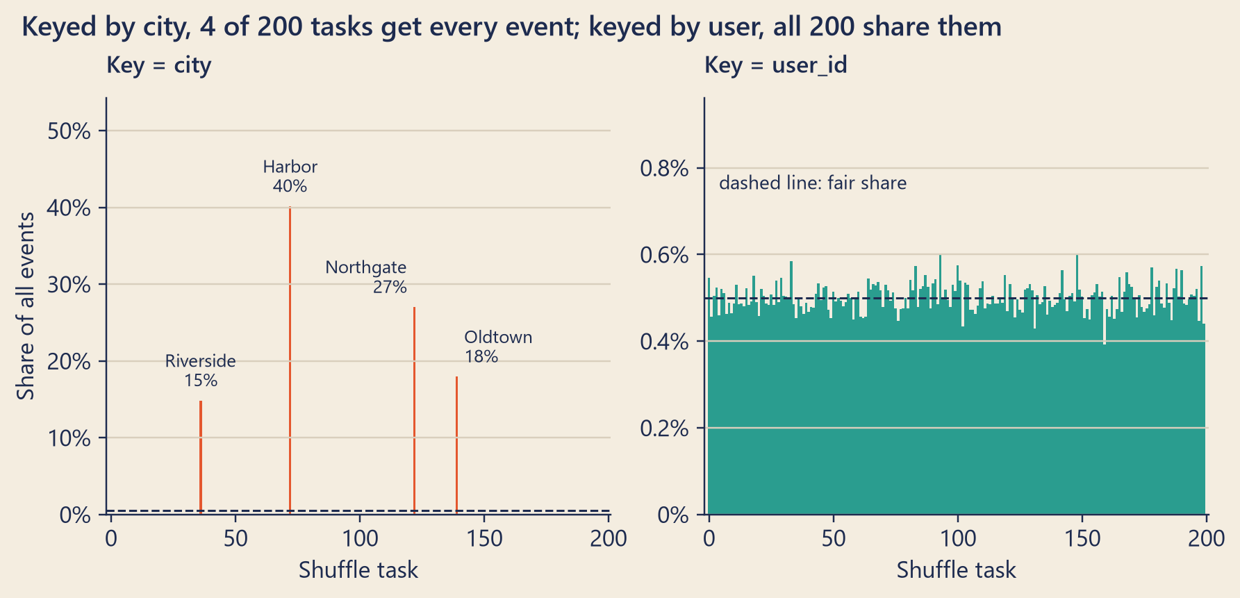
Mia’s window function said PARTITION BY city. So the key of her shuffle was the city. There were four keys. In a stage of 200 tasks, only four tasks received any rows. The other 196 had nothing to do.
Show the code
bk.setup()fig, (left, right) = plt.subplots(1, 2, figsize=(8, 3.8), layout="constrained")x = np.arange(SHUFFLE_PARTITIONS)left.bar(x, tasks_city / n_events, width=1.0, color=bk.TOMATO)for c, t in city_task.items():# Two cities can sit on nearby tasks: push their labels apart, left and right. near = [u for o, u in city_task.items() if o != c andabs(u - t) <25] ha ="center"ifnot near else ("right"if t < near[0] else"left") dx = {"center": 0, "right": -3, "left": 3}[ha] left.text(t + dx, city_share[c] +0.012, f"{display[c]}\n{bk.fmt_pct(city_share[c], 0)}", ha=ha, va="bottom", fontsize=8.5, color=bk.INK)left.set_ylim(0, harbor_share *1.35)right.bar(x, tasks_user / n_events, width=1.0, color=bk.TEAL)right.set_ylim(0, user_task_max *1.6)for ax, title in ((left, "Key = city"), (right, "Key = user_id")): ax.axhline(1/ SHUFFLE_PARTITIONS, color=bk.INK, linestyle="--", linewidth=1) ax.set_title(title, fontsize=11) ax.set_xlabel("Shuffle task") ax.set_xlim(-2, SHUFFLE_PARTITIONS +1) ax.yaxis.set_major_formatter(lambda v, _: "0%"if v ==0elsef"{v:.1%}"if v <0.02elsef"{v:.0%}")left.set_ylabel("Share of all events")right.text(4, user_task_max *1.25, "dashed line: fair share", fontsize=9, color=bk.INK)fig.suptitle(f"Keyed by city, {busy_tasks} of {SHUFFLE_PARTITIONS} tasks get every event; "f"keyed by user, all {SHUFFLE_PARTITIONS} share them", x=0.01, ha="left", fontsize=13, fontweight="semibold", color=bk.INK)plt.show()
Figure 1: The rows each of the 200 shuffle tasks receives in Mia’s job. Left: the key is the city. Right: the key is the user (note the much smaller scale). Adaptive execution is off, as it was on Steep’s cluster. The hash function here is Murmur3, the same family that Spark uses.
When a few keys hold far more rows than the others, the work is uneven. This is data skew, and a key with far too many rows is a hot key. Here, Harbor is the hot key. You met it in Chapter 8: keyed by city, Kafka would have had a hot partition. On Monday 14 September alone, 39% of the events came from Harbor; since June, 40%.
A job is as slow as its slowest task. Harbor’s task held 40.2% of all events. So, even with a thousand machines, this step of the job could never run more than 2.5 times faster than on one machine alone: 1 divided by 0.40. Worse, Harbor’s task had more rows than its executor could hold in memory. It spilled to disk again and again, so it ran far longer than its share alone suggests. That is how three cities finished in minutes and Harbor took hours.
Skew does not hurt every query. Suppose Mia had only counted events per city. Spark and Hive would first count inside each task, as the map workers did on the napkin, and the shuffle would carry a few numbers per task. The hot key would hardly matter. Skew hurts when one task must see every row of its key: windows and sorting (as in Mia’s job), joins, and collecting values into a list.
Joins have a famous hot key of their own: NULL. Of the 6.7 million events since June, 89% have no order_id, because only order_completed events carry one. Suppose you keep every event and LEFT JOIN it to the orders on order_id. If the join shuffles, every row with a NULL key gets the same hash, and they all land on one task.
Five fixes
1. Split by the real unit of work. Mia’s question was about each user’s next event, not each city’s. Theo changed one line, from PARTITION BY city to PARTITION BY user_id. Now there were 82,798 keys, and every task got between 0.39% and 0.60% of the events, close to the fair share of 0.50%. The count by city moved to the last step, where the map-side counts keep it small. The new job finished in minutes. It was also correct, which the first job was not. With the city as the partition and the rows in time order, the “next event” was the next event from anyone in that city, usually another customer.
-- For each checkout since 1 June: what was the same user's next event?WITH steps AS (SELECT u.city, e.event_name, e.event_date,LEAD(e.event_name) OVER (PARTITIONBY e.user_id -- was: PARTITION BY u.cityORDERBY e.event_time ) AS next_eventFROM dwd_event_detail AS eJOIN ods_users AS u ON u.user_id = e.user_idWHERE e.event_date >=DATE'2026-06-01')SELECT city, event_date >=DATE'2026-09-07'AS from_7_sep,avg(CASEWHEN next_event ='order_completed'THEN1ELSE0END) AS completed_nextFROM stepsWHERE event_name ='checkout_start'GROUPBY1, 2;
2. Salt the hot key. Sometimes the hot key must stay, for example in a join between two big tables on a key with one very common value. Then you salt it: add a small random number to the key, so one hot key becomes several smaller ones. harbor becomes harbor_0, harbor_1, … harbor_7. Each piece holds about one eighth of Harbor’s rows and can go to a different task. A second, small step then puts the pieces together again. Salting works only when the work can be done in pieces and put back together: a join (copy the other side once per salt), a distinct count in two steps, or a list of values. It cannot fix a window like LEAD by city, because each row needs its true neighbour.
3. Broadcast the small table. Mia’s job looked up each user’s city in the users table. That table is small. Instead of shuffling both sides of the join, Spark copies the small table to every executor, and each task joins its own events locally. This is a broadcast join (Hive calls it a map join). The big table never moves. By default, Spark broadcasts a table automatically when it believes the table is smaller than 10 MB.
4. Treat hot keys apart. Rows with a NULL key can never match, so send them around the join: join only the rows that have a key, and add the others back with UNION ALL. In the same way, a known hot key, such as Harbor or a test account, can get its own small job, with the results put together at the end.
5. Let the engine help. Since version 3.2, Spark turns on adaptive query execution (AQE) by default. It looks at the real sizes of the data while the job runs, and changes the plan. It can merge tiny tasks, switch to a broadcast join, and cut a skewed join into smaller tasks. With AQE on, Spark would have merged the 196 empty tasks away. Harbor would still be one task. In a join, Harbor’s rows can be cut into pieces, each matched with a copy of the other table. A window cannot be cut.
NoteUnder the hood
Choosing a task. Spark’s shuffle sends a row with key \(k\) to task
where \(h\) is the Murmur3 hash with seed 42, \(N\) is the number of shuffle partitions, and pmod is a remainder that is never negative. The figure and the simulator use the standard 32-bit Murmur3 with seed 42 and, as Spark does, take pmod of the hash read as a signed number. Spark’s own Murmur3 treats the last few bytes of a string slightly differently, so its exact task numbers can differ. The pattern does not.
The slowest task sets the time. If task \(i\) receives \(W_i\) rows and every executor handles \(v\) rows per second, the stage takes about
where \(p_{\max}\) is the share of the biggest key. For Mia’s first job, \(p_{\max}\) = 0.402, so the speed-up can never pass 2.49. This ignores spilling, which makes the biggest task even slower.
Salting. Split a key with share \(p\) into \(S\) pieces, and each piece holds about \(p/S\). For a join, salt the big side with a random number from 0 to \(S-1\), and copy each row of the other side \(S\) times, once for each salt value, so that every piece still finds its partner. For a distinct count, take the salt from the counted value itself, such as \(\text{hash}(\text{user\_id}) \bmod S\), so that each value lands in exactly one piece. Count the distinct values of each (key, salt) piece, then add up the pieces. A plain sum or count needs no salt in Spark or Hive: partial aggregation already does the work in pieces. With \(S = 8\), Harbor’s pieces hold about 5.0% each. But 32 salted keys still land on 8 workers by hash, and some workers get more pieces than others: the slowest worker then holds 22%.
AQE in detail. AQE merges small shuffle partitions after the shuffle, switches a sort-merge join (a common kind of shuffle join) to a broadcast join when one side turns out small, and splits skewed partitions in a sort-merge join. In a sort-merge join, Spark treats a shuffle partition as skewed when it is larger than 5 times the median partition and larger than 256 MB. (The settings are skewedPartitionFactor and skewedPartitionThresholdInBytes, both under spark.sql.adaptive.skewJoin.) It then splits that partition and copies the matching part of the other side.
Distinct counts. In Hive, an exact COUNT(DISTINCT …) per key can be skewed too, because one task gets every value of a hot key. Spark first groups by the key and the counted value together, which spreads that work.
Hive’s engines. At first, Hive turned each SQL query into MapReduce jobs. Later versions run on faster engines, such as Apache Tez.
Hive’s settings.hive.map.aggr (on by default) aggregates on the map side. hive.groupby.skewindata (off by default) runs a GROUP BY as two jobs, first spreading rows at random, then combining. hive.optimize.skewjoin (off by default) handles very frequent join keys in a separate step. hive.auto.convert.join (on by default since Hive 0.11) turns a join with a small table into a map join. Hive’s settings for skew are off by default.
Small files in Hive and Spark (Chapter 9). When writing: control how many tasks write each partition (set the number of reducers, the tasks of the reduce step, or DISTRIBUTE BY the partition column in Hive, or repartition in Spark). hive.merge.mapfiles (on by default) merges the output of jobs that have only a map step; hive.merge.mapredfiles (off by default) must be turned on for jobs with a reduce step. For ORC tables, ALTER TABLE … CONCATENATE merges small files stripe by stripe, without decoding the data. When reading: Hive’s default input format, CombineHiveInputFormat, packs small files into one task. Spark packs files into one task up to its maxPartitionBytes setting (128 MB by default), counting 4 MB for each file it opens.
HDFS placement. With three copies, HDFS puts one copy on the writer’s own machine if it is a DataNode (otherwise on a machine in the writer’s rack), and the other two on two different machines in one other rack (a cabinet of servers that share a network switch). One whole rack can fail and a copy survives.
What the fixed job found
The new job also answered Mia’s question from Wednesday. From 1 June to 6 September, the next event after a checkout was order_completed between 78% and 79% of the time, week after week, and about 78% in every city. From 7 September, the share fell by 11 to 12 points, in all four cities at once. So the gap was new. It began on the day her small charts had shown (Chapter 5), and nothing like it happened earlier in the summer.
Then she tested the second word in her notebook, computing. The dashboard’s daily orders come out of jobs like hers. She counted the order_completed events in the raw lake files herself, day by day, and compared her counts with the dashboard. On all 114 days from 1 June to 22 September, the largest difference was 0. (She left out 23 September: that row was built early that morning, before all of the day’s late events had arrived.) The jobs did exactly what they were told. The missing events were never in the lake.
Try it
The data-skew simulator. These are the real events since 1 June, in this book’s sample. Choose how many workers share the job and which key the shuffle uses. Each bar is one worker. The job ends when the slowest worker (in tomato) ends.
Show the code
skewSimulator = {const D =JSON.parse(document.getElementById("ch10-sim").textContent);const C = {teal:"#2a9d8f",tomato:"#e4572e",tomatoText:"#b8401c",mustard:"#f2b134",ink:"#1d2b4f",paper:"#f4ede0",grid:"#d9cfbd",muted:"#5f6475"};const KEYS = ["city","user_id","city + salt"];// Murmur3 (x86, 32-bit) with seed 42: the hash family Spark uses to pick a shuffle task.functionmurmur3(text, seed =42) {const data =newTextEncoder().encode(text);const n = data.length, nb = n - (n %4);const c1 =0xcc9e2d51, c2 =0x1b873593;let h = seed >>>0, k;for (let i =0; i < nb; i +=4) { k = data[i] | (data[i +1] <<8) | (data[i +2] <<16) | (data[i +3] <<24); k =Math.imul(k, c1); k = (k <<15) | (k >>>17); k =Math.imul(k, c2); h ^= k; h = (h <<13) | (h >>>19); h = (Math.imul(h,5) +0xe6546b64) |0; } k =0;for (let j = n - nb -1; j >=0; j--) k = (k <<8) | data[nb + j];if (n > nb) { k =Math.imul(k, c1); k = (k <<15) | (k >>>17); k =Math.imul(k, c2); h ^= k; } h ^= n; h ^= h >>>16; h =Math.imul(h,0x85ebca6b); h ^= h >>>13; h =Math.imul(h,0xc2b2ae35); h ^= h >>>16;return h >>>0; }const pmod = (h, n) => ((h % n) + n) % n;// a remainder that is never negativeconst workersIn = Inputs.range([1, D.maxWorkers], {step:1,value: D.defaultWorkers,label:"Workers"});const keyIn = Inputs.radio(KEYS, {value:"city",label:"Shuffle key"});const saltIn = Inputs.range([2,16], {step:1,value: D.defaultSalt,label:"Salt pieces per city"});const svgBox = htl.html`<div class="sk-svg"></div>`;const statsBox = htl.html`<div class="sk-stats"></div>`;const noteBox = htl.html`<div class="sk-note" aria-live="polite"></div>`;functionloads(n, key, salt) {const out =Array.from({length: n}, () => ({rows:0,keys: []}));if (key ==="user_id") { D.userLoads[String(n)].forEach((v, i) => { out[i].rows= v; });return out; }for (const [name, label, rows] of D.cities) {const pieces = key ==="city"?1: salt;for (let s =0; s < pieces; s++) {const w =pmod(murmur3(pieces ===1? name :`${name}_${s}`) |0, n);// as Spark: signed hash out[w].rows+= rows / pieces; out[w].keys.push(label); } }return out; }const hours = h => {const total =Math.round(h *60);return total >=60?`${Math.floor(total /60)} h ${total %60} min`:`${total} min`; };const pct = (x, d =1) =>`${(100* x).toFixed(d)}%`;const keyText = (keys, key, band) => {if (key !=="city") returnString(keys.length);// salted: how many pieces landed hereif (keys.length===1&& band >=60) return keys[0];// room for the full city namereturn keys.map(k => k.slice(0,1)).join("+");// initials when space is short };let W =640;// drawing width; follows the page width, so text keeps its real size on phonesfunctionrender() {const n = workersIn.value, key = keyIn.value, salt = saltIn.value; saltIn.style.opacity= key ==="city + salt"?1:0.45;const ws =loads(n, key, salt);const total = D.total;const max =Math.max(...ws.map(w => w.rows));const slowest = ws.findIndex(w => w.rows=== max);const idle = ws.filter(w => w.rows===0).length;const H =230, LEFT =40, BOTTOM =34, TOP =12;const top =Math.max(0.45, (max / total) *1.12);const y = v => TOP + (H - TOP - BOTTOM) * (1- v / top);const band = (W - LEFT -6) / n, bw =Math.max(2, band *0.72);const shapes = []; [0,0.1,0.2,0.3,0.4,0.5,0.6,0.7,0.8,0.9,1].filter(t => t <= top).forEach(t => { shapes.push(htl.svg`<line x1="${LEFT}" x2="${W -4}" y1="${y(t)}" y2="${y(t)}" stroke="${C.grid}" stroke-width="1"/>`); shapes.push(htl.svg`<text x="${LEFT -6}" y="${y(t) +4}" text-anchor="end" font-size="12" fill="${C.muted}">${Math.round(100* t)}%</text>`); }); ws.forEach((w, i) => {const x = LEFT + i * band + (band - bw) /2;const share = w.rows/ total; shapes.push(htl.svg`<rect x="${x}" y="${y(share)}" width="${bw}" height="${Math.max(0,y(0) -y(share))}" fill="${i === slowest ? C.tomato: C.teal}" rx="2"/>`);if (band >=26) { shapes.push(htl.svg`<text x="${x + bw /2}" y="${H - BOTTOM +15}" text-anchor="middle" font-size="12" fill="${C.ink}">W${i +1}</text>`);if (key !=="user_id") { shapes.push(htl.svg`<text x="${x + bw /2}" y="${H - BOTTOM +29}" text-anchor="middle" font-size="11" fill="${w.rows? C.ink: C.muted}">${w.rows?keyText(w.keys, key, band) :"idle"}</text>`); } } });const fair =1/ n; shapes.push(htl.svg`<line x1="${LEFT}" x2="${W -4}" y1="${y(fair)}" y2="${y(fair)}" stroke="${C.ink}" stroke-dasharray="5,4" stroke-width="1.3"/>`); shapes.push(htl.svg`<text x="${W -6}" y="${y(fair) -5}" text-anchor="end" font-size="12" fill="${C.ink}">fair share</text>`); svgBox.replaceChildren(htl.svg`<svg viewBox="0 0 ${W}${H}" width="100%" role="img" aria-label="${n} workers, key ${key}: the slowest worker holds ${pct(max / total)} of the events; fair share ${pct(fair)}" style="max-width:${W}px;font-family:Inter,system-ui,sans-serif">${shapes}</svg>`);const t = D.oneWorkerHours* max / total;const tFair = D.oneWorkerHours/ n; statsBox.replaceChildren(htl.html`<div><strong>Slowest worker:</strong> ${pct(max / total)} of all events (fair share ${pct(fair)}). <strong>Idle workers:</strong> ${idle} of ${n}.</div> <div><strong>Job time:</strong> ${hours(t)}, if one worker alone needs ${D.oneWorkerHours} hours (perfect split: ${hours(tFair)}). <strong>Speed-up:</strong> ×${(total / max).toFixed(1)} of a possible ×${n}.</div>`);let note ="";if (key ==="city") {const used = ws.filter(w => w.rows>0).length; note = used <Math.min(n, D.cities.length)?"Two or more cities landed on the same worker by chance. With only four keys, such collisions are common.":`Only ${D.cities.length} keys exist, so at most ${D.cities.length} workers get work. Harbor's worker sets the pace, however many workers you add.`; } elseif (key ==="user_id") { note ="Tens of thousands of users spread almost evenly over the workers. This is the fix Theo used."; } else { note =`Each city is split into ${salt} pieces; the number under a bar is how many pieces that worker got. `+"A second, small step puts the pieces together again. This works for joins, distinct counts and lists. "+"It would not fix Mia's window, because each row needs its true neighbour."; } noteBox.textContent= note; }for (const input of [workersIn, keyIn, saltIn]) input.addEventListener("input", render);render();const resizer =newResizeObserver(() => {const next =Math.max(300,Math.min(640,Math.round(svgBox.clientWidth) ||640));if (next !== W) { W = next;render(); } }); resizer.observe(svgBox); invalidation.then(() => resizer.disconnect());const style =document.createElement("style"); style.textContent=` .sk-wrap { font-family: Inter, system-ui, sans-serif; color: ${C.ink}; } .sk-controls { display: flex; flex-wrap: wrap; gap: 0.2rem 1.5rem; align-items: flex-start; } .sk-stats, .sk-note { font-size: 0.85rem; margin-top: 0.4rem; } .sk-note { min-height: 2.6em; color: #3d4766; }`;return htl.html`<div class="sk-wrap">${style} <div class="sk-controls">${workersIn}${keyIn}${saltIn}</div>${svgBox}${statsBox}${noteBox} </div>`;}
Things to try:
Keep 8 workers and the key city. The slowest worker holds 40%. Add workers: the job does not get faster, and more workers sit idle. With 10 workers it even gets slower: two cities land on one worker, which then holds 67%.
Try 6 workers. By chance, three cities land on the same worker.
Switch the key to user_id. With 8 workers, the slowest holds 12.7%, almost exactly the fair share. Now more workers really do help.
Switch to city + salt with 8 pieces. The slowest worker drops to 22%. Raise the pieces to 16: it falls to 18%. (Not every step helps: the pieces still land on workers by hash.)
The simulator simplifies. Each worker reads the same number of rows per second, the job time is set by the slowest worker alone, and nothing spills. Real skew is usually worse than this.
Common traps
Adding machines to a skewed job. If one key holds 40% of the rows, as Harbor does, that step of the job cannot run more than 2.5 times faster than on one machine, however big the cluster.
Raising the number of shuffle partitions to fix one hot key. More partitions split the other keys more finely. The hot key still lands, whole, on one task.
Forgetting NULL. Missing join keys hash to the same value and pile up on one task.
Dropping an external table and expecting the files to go. They stay. Dropping a managed table deletes them.
Writing files and expecting Hive to see them. A new partition folder is invisible until it is added to the metastore.
Trusting schema-on-read. A bad file loads without complaint and shows up later as NULLs.
TipAudit Instinct · Split the fieldwork, and split the giant
A group audit is split across teams by entity: one team per subsidiary. The audit is finished only when the last team is finished. If one subsidiary holds almost half of the group’s revenue, its team is the slowest, and adding teams to the small subsidiaries does not help.
Good audit managers do not wait. They split the big entity: one team for its sales cycle, one for purchases, one for payroll. Then they put the results together at group level. That is salting, done with people.
Two more habits carry over. Plan the split from the size of each entity, not from the number of entities. And watch for the entity that cannot be split, such as one huge contract, and give it its own team early.
NoteInterview Corner
Q1. How do you handle data skew in Hive or Spark?
NoteA short answer
First, confirm it: in the Spark UI, compare the slowest task with the median task (time and shuffle read size), then count rows per key to find the hot keys. Then fix the cause. Use a better key if the question allows (for example, user instead of city). Filter or separate NULLs and other hot keys. Broadcast small tables (map join in Hive). Salt hot keys when the work can be put back together: for joins, a random salt on the big side and copies of the other side; for distinct counts, a salt taken from the counted value. Rewrite COUNT(DISTINCT x) as a GROUP BY on the key and x, followed by a COUNT. Check that join keys have the same type: casting text keys to numbers can turn them into NULLs, which then pile up on one task. In Spark 3, AQE (on by default since 3.2) splits skewed partitions in sort-merge joins. In Hive, hive.map.aggr, hive.groupby.skewindata and hive.optimize.skewjoin. More partitions alone do not help a single hot key.
Q2. What is the difference between internal (managed) and external Hive tables?
NoteA short answer
For a managed table, Hive owns the data: DROP TABLE deletes the metadata (the table’s description in the metastore) and the files (the files may go to the trash first). Some features, such as ACID transactions and TRUNCATE, work only on managed tables. For an external table, Hive owns only the metadata: DROP TABLE leaves the files in place. Use external tables for raw data that other jobs write or other teams share, and run MSCK REPAIR TABLE (or ALTER TABLE … ADD PARTITION) when new partition folders appear. Use managed tables for data whose whole life Hive should control. Two details: since Hive 4.0, the table property external.table.purge makes DROP delete an external table’s files too. And in Hive 3 and later, many installations make a plain CREATE TABLE a transactional (ACID) managed table, so check with DESCRIBE FORMATTED.
Q3. What triggers a shuffle in Spark?
NoteA short answer
Any step that needs rows with the same key in the same place: aggregations by key (groupBy, reduceByKey), joins (unless one side is broadcast, or both sides are already partitioned the same way), distinct, window functions with PARTITION BY, a global sort, and repartition. Each shuffle ends a stage. Steps such as select, filter and map do not shuffle: each task works on its own slice. Fewer and smaller shuffles make faster jobs.
Reported change: −12.0% orders, the week of 7 September compared with the week before (CEO dashboard).
Explained so far: 0 of the 12 points. About 7 of them sit between the orders database and the dashboard (Clue 1).
Suspects: the iOS app, version 3.2.0 (Chapter 6): the main suspect, not proved. The service that writes app events to Kafka (Chapter 8): a minor suspect.
Ruled out: the matcha menu (Chapter 4), Kafka (Chapter 8), storage (Chapter 9), and now computing (Chapter 10).
Open questions: Can late changes to orders, such as refunds, move the numbers? (Chapter 11.) Did iOS 3.2.1, released this morning, close the gap? What exactly broke, and how many points does it explain? (Chapter 15.)
New evidence: recounted from the raw lake files, the dashboard is right about the events it has: on 114 days, the largest difference was 0. The gap is new: all summer, the next event after a checkout was order_completed 78% to 79% of the time; from 7 September it fell by about 12 points in every city. iOS 3.2.1 went out at 06:00 on 24 September, labelled Bug fixes and improvements. Not yet tested.
Recap
When data is too big for one machine, split the data (HDFS blocks with copies, or object storage) and split the work (map, shuffle, reduce). Hive adds a table on top of files: a metastore with schemas, locations and partitions.
Spark runs the same idea faster: a lazy plan, stages cut at shuffles, one task per slice, data kept in memory when it fits.
A job is as slow as its slowest task. Choose shuffle keys with many, even values; salt, broadcast or separate hot keys; and let AQE split skewed joins.
English
中文
distributed
分布式
cluster / node
集群 / 节点
scale up / scale out
纵向扩展 / 横向扩展
HDFS
分布式文件系统
block
数据块
replication factor
副本因子
NameNode / DataNode
名称节点 / 数据节点
data locality
数据本地性
object storage
对象存储
metastore
元数据存储
schema-on-read
读时模式
managed (internal) table
管理表(内部表)
external table
外部表
MapReduce
MapReduce(映射-归约)
combiner
合并器(map 端预聚合)
driver / executor
驱动器 / 执行器
task / stage
任务 / 阶段
lazy evaluation
惰性求值
shuffle
洗牌 / 数据重分布
data skew
数据倾斜
hot key
热点键
salting
加盐
broadcast join (map join)
广播连接(map join)
adaptive query execution
自适应查询执行
Further reading
Jeffrey Dean and Sanjay Ghemawat, “MapReduce: simplified data processing on large clusters”, Communications of the ACM 51(1), 2008. doi:10.1145/1327452.1327492.
Ashish Thusoo and others, “Hive: a warehousing solution over a map-reduce framework”, Proceedings of the VLDB Endowment 2(2), 2009. doi:10.14778/1687553.1687609.
Matei Zaharia and others, “Apache Spark: a unified engine for big data processing”, Communications of the ACM 59(11), 2016. doi:10.1145/2934664.