9 · Rows, Columns, and Indexes: How Data Is Stored
On Wednesday morning, Mia read her notes from Tuesday. Kafka was cleared: the missing order_completed events had never reached it. Why keep following the order, then? Because the dashboard’s numbers pass through more stops after Kafka: the data lake that stores the events, and the jobs that turn them into the dashboard. If any of those stops also lost events, part of the gap would belong to them. To say that the whole gap belongs to the app side, Mia had to show that nothing more is lost further down the line. An auditor tests every stop on the path, not only the first one that fails. She wrote two words in her notebook: storage and computing.
But first, she wanted to look further back in time. Her small charts from last Friday started on 10 August. In every city, the dashboard had begun to miss orders on 7 September (Chapter 5). Had the same thing happened earlier in the summer, on a smaller scale? If the gap was new, something had changed in September. If it was old, she was looking at the wrong week.
She already had the dashboard’s daily numbers. She needed the other side: the orders in the database, day by day since 1 June, by platform, app version, payment method and status. Then she could lay the two lines side by side for the whole summer. She still had the read access to the orders database that Theo had given her in her first week. Until now, her questions had covered a week or two. She pressed “Run” at 10:14.
The query ran. And ran.
At 10:15, a message appeared in the operations chat: “Checkout is slow in all four cities. Is anyone releasing a new version?”
At 10:16, Theo was standing behind her chair. He looked at her screen. “May I?” He stopped her query. A minute later, the operations chat said: “Back to normal.”
Mia’s face was hot. “I broke checkout.”
“You slowed it down for two minutes,” said Theo. “No order was lost. And the mistake is mine, not yours. I gave you a key to the cash register. I should have given you a key to the library.”
He sat down and took two napkins from his drawer.
“Your query did not change anything,” he said. “It only read. But it read every order we have ever taken, and it read each one whole. While the database worked on your question, it had less time for customers. Checkout and your query share the same processors, the same memory and the same disks.”
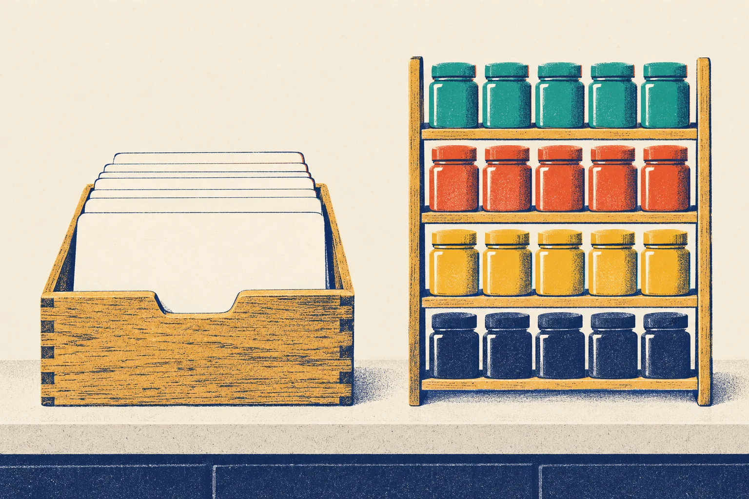
On the first napkin, he drew a box of recipe cards. On the second, a spice rack.
“There are two ways to keep the same data,” he said. “You asked your question to the wrong one.”
Mia wrote at the top of a new page: Why did a query that only reads slow down checkout? Where should a question like mine go? Her question about the summer would have to wait until Thursday (Chapter 10).
ImportantThe big idea
How data is stored decides which questions are cheap. An index finds a few rows fast; analysis wants columns, not rows.
Look at the picture: on the left, a box of recipe cards; on the right, a spice rack where each shelf holds one kind of spice. Both can hold the same information. By the end of this chapter, you will know why a big question belongs on the right.
Two kinds of work
Think of a Steep store at lunchtime. The cash register asks the system small questions, very fast, all day: save this order, find order 4158971, mark it as paid. Each question touches one order. Each must finish in a few milliseconds, because a customer is waiting.
Now think of the manager on a Friday. She asks a different kind of question: how many orders did we have each day since June? It is one question, but it touches every order.
Work of the first kind is called OLTP, short for online transaction processing. It means many small reads and writes, each about one record, each fast. A transaction here is one unit of business work, such as saving an order together with its payment. Steep’s orders database does OLTP work. It is also production: the live system that customers use right now.
Work of the second kind is called OLAP, short for online analytical processing. It means a few big questions, each reading a large part of the data and summing it up.
The two kinds of work fight when they share one machine. Mia asked a big analysis question of the live system that serves customers. The orders table had no index on the order time. (An index is a sorted list that lets a database jump to the right rows, like the index at the back of a book. More on indexes below.) So the database read every order Steep had ever taken, not only the ones since June. Order numbers count up from Steep’s first order, and that morning they had passed 4,216,843. So the query read about 4.2 million orders to answer a question about 0.74 million: the orders from 1 June to that Tuesday. (The copy of the data that comes with this book keeps only those.)
That is why companies copy their data out of production. They send it to a separate place built for big questions. That can be a read replica, which is a read-only copy of the database on another machine. It can also be a data lake or a data warehouse. Steep’s data lake already held a copy of every order. Mia should have asked there.
Finding one order fast: indexes and the B+ tree
Mia still had a question. “At the counter, the staff type an order number, and the order is there at once. Why could the same database not answer me?”
“Because it has an index for their question,” said Theo, “and none for yours.”
What an index is. Picture a library with a million books. To find one book by its title, you do not walk along every shelf. You go to the card catalogue: drawers of cards, sorted by title, where each card says where the book stands. An index in a database is the same idea. It is a sorted copy of one or more columns, and each entry points to its row. A lookup becomes a few jumps instead of a read of everything. The column that an index is sorted by is its index key.
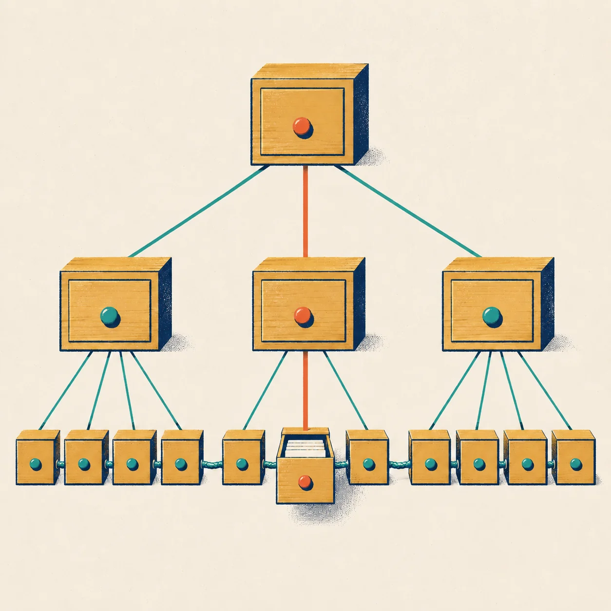
The B+ tree. A database keeps its data on disk in blocks of one fixed size, called pages. Steep’s orders database is MySQL, and its storage engine, InnoDB, uses pages of 16 KB by default. The pages of an index form a tree, like the card catalogue in the picture below. The leaf pages at the bottom hold the keys in order, and each leaf is linked to its neighbours on both sides. The pages above hold only signposts, such as “order numbers from 4,150,000 to 4,200,000: go down here”. To find one order, the database reads the top page, the root, follows one signpost on each level, and arrives at the right leaf. This shape is called a B+ tree. (MySQL’s documentation calls it a B-tree. Strictly, it is the variant that textbooks call a B+ tree. The box “Under the hood” explains the difference.)
The trick is the width. A 16 KB page holds hundreds of signposts, so the tree stays very short. Here is a rough estimate for Steep’s orders table that morning, with about 4.2 million rows. Suppose one order takes about 200 bytes, one signpost about 16 bytes, and pages are about 15/16 full, as InnoDB leaves them when rows arrive in order. Then a leaf page holds about 76 orders, and a signpost page holds about 960 signposts. The tree has three levels: one root page, 58 pages below it, and about 55,000 leaf pages. Three page reads find any one order among 4.2 million. In practice, the top levels stay in memory, so at most one read touches the disk, and often none.
A range, such as all orders numbered from 4,150,000 to 4,151,000 (or, with an index on the order time, all orders from 8:00 to 9:00), works almost the same way. The database finds the first matching leaf, then walks along the linked leaves until the range ends.
Mia’s query, with no index on the order time, read every leaf page: about 55,000 pages, or about 0.9 GB.
Two kinds of index. In InnoDB, the table itself is a B+ tree. Its key is the primary key, the column that names each row (for Steep’s orders, order_id), and its leaf pages hold the whole rows. This tree is the clustered index: the rows are stored in key order. Every other index on the table is a secondary index. Its leaf entries hold the indexed column and the primary key, not the row. So a lookup through a secondary index often needs a second trip. Suppose Steep indexes user_id, and the app’s order-history screen asks for all of Mia’s orders. The secondary index gives her order numbers. Then, for each one, the database searches the clustered index for the row. Chinese engineers call this second trip 回表, “back to the table”. If an index already holds every column a query needs, there is no second trip: the index is a covering index for that query.
Indexes on several columns. An index can be sorted by more than one column, like a phone book sorted by family name and then by given name. This is a composite index. Suppose Steep indexes (store_id, created_at). A query for one store in one hour can use both columns. A query for one store alone can use the first column. But a query for one hour across all stores often cannot use it, in the same way that a phone book sorted by family name does not help you find everyone called Mia. This is the leftmost-prefix rule (最左前缀): an index helps with its first column, with its first two columns, and so on, but not with a later column on its own.
The price of an index. Every index is a second copy of some columns, kept in order. Each new order must be added to the table and to every index. Each change must also update every index that holds a changed column. More indexes mean slower writes and more disk space. So a busy OLTP table has a few well-chosen indexes, for the questions it hears all day.
Why an index would not have saved Mia. With an index on the order time, the database could skip the orders before June. But her question still touched 0.74 million of the 4.2 million orders, 17% of the table, and it would still read each of those rows whole, with all 17 columns. When a query touches a large share of a table, reading the pages in order is often faster than jumping through an index, so the database often chooses a full scan anyway. And her next question, by store or by hour, would need yet another index. Indexes make it cheap to find a few rows. Analysis reads a few columns of many rows. For that, the data needs a different shape: Theo’s napkins.
Other shapes. An LSM tree (log-structured merge tree) collects new writes in memory, writes them out as sorted files, and merges those files in the background. Writes are very fast, so systems with heavy writes use it: RocksDB, HBase and Cassandra, and Paimon in Chapter 11. A hash index turns each key into a position with a fixed formula (a hash, Chapter 8). It finds one exact key very fast, but it cannot find a range, because neighbouring keys land far apart.
NoteUnder the hood: B+ trees and their rivals
B-tree and B+ tree. In the original B-tree (Bayer and McCreight, 1972), every page, at every level, holds keys together with their data: the record, or a pointer to it. A B+ tree keeps the records, or pointers to them, only in the leaves, and links the leaves in key order. The signpost pages then hold only keys and page numbers, so more of them fit on a page: a higher fan-out, the number of children per page. A range scan walks along the leaves without climbing back up. In InnoDB, the pages on each level of an index form a doubly linked list, and the leaves of the clustered index hold the rows.
Height. With \(n\) rows, \(r\) rows per leaf page and a fan-out of \(f\), the tree has
\[h = 1 + \Big\lceil \log_f \big\lceil n / r \big\rceil \Big\rceil\]
levels. For the estimate above, \(n \approx\) 4.2 million, \(r =\) 76 and \(f =\) 960: there are 55,485 leaf pages, \(\log_f\) of that is 1.59, which rounds up to 2, so \(h =\) 3.
Why not a binary tree, or a hash? A binary tree gives each node two children, so it is about \(\log_2 n\) levels deep: 23 levels for 4.2 million keys, and each level can cost a page read. A hash finds an exact key in one step, but it keeps no order: no ranges, no ORDER BY, no leftmost prefix. (InnoDB can also build a small hash index on top of its B-trees by itself, the adaptive hash index, for lookups it sees often. Since MySQL 8.4 this feature is off unless you switch it on.)
LSM trees. New writes go to a sorted table in memory and to a log on disk. When the memory table is full, it is written to disk as a sorted file. In the background, compaction merges small sorted files into bigger ones. The costs move around. Each row is rewritten several times as files merge (write amplification), and one read may have to check several files (read amplification). Bloom filters reduce that for single-key lookups, not for ranges. O’Neil and others described the design in 1996.
When an index often cannot be used. Optimisers differ between databases and versions, so read these as “often”:
a function on the column, such as WHERE DATE(created_at) = …. Write a range on the column instead, or, in MySQL 8, index the expression itself;
a LIKE pattern that starts with a wildcard, such as LIKE '%1024' (LIKE 'A10%' can use the index);
a type conversion: a text column compared with a number, such as user_id = 1. Many strings turn into the same number, so MySQL cannot use the index;
a skipped leftmost column. MySQL 8 can sometimes use a skip scan, one small search for each value of the first column, but only when the query needs no column outside the index and the first column has few values;
columns after a range condition (>, <, BETWEEN, LIKE) in the same index: they no longer narrow the search;
OR across different columns: one index cannot answer it, so MySQL merges two indexes or scans the table;
a query that touches a large share of the table: reading every page in order is often cheaper.
The B+ tree explorer. This toy tree holds the 5,711 orders of Monday 14 September. Type an order number (order_id, not the pickup code) or press a button. The explorer follows the signposts down to a leaf and counts the pages it reads. Each entry on a page is either a signpost to one page below or, on a leaf, one order. Its pages hold only a few entries; a real InnoDB page holds hundreds.
Show the code
btreeExplorer = {const T =JSON.parse(document.getElementById("ch09-tree").textContent);const C = {teal:"#2a9d8f",tealText:"#1f7a6f",tomato:"#e4572e",tomatoText:"#b8401c",mustard:"#f2b134",ink:"#1d2b4f",paper:"#f4ede0",grid:"#d9cfbd",muted:"#5f6475"};const N = T.count, FIRST = T.first, LAST = T.first+ T.count-1;const fmt = n => n.toLocaleString("en-US");const plural = (n, word) =>`${fmt(n)}${word}${n ===1?"":"s"}`;const idIn = Inputs.text({label:"Order number (order_id)",value:String(T.mia)});const fanIn = Inputs.range([3,64], {step:1,value:8,label:"Entries per page"});const rangeIn = Inputs.range([1,2000], {step:1,value:200,label:"Orders in a range"});const svgBox = htl.html`<div class="bt-svg"></div>`;const pathBox = htl.html`<ol class="bt-path"></ol>`;const statsBox = htl.html`<div class="bt-stats" aria-live="polite"></div>`;let W =640;// drawing width; follows the page widthfunctionlevelSizes(F) { // pages per level: leaves first, the root lastconst sizes = [Math.ceil(N / F)];while (sizes[sizes.length-1] >1) sizes.push(Math.ceil(sizes[sizes.length-1] / F));return sizes; }const firstKey = (F, level, page) => FIRST + page * F ** (level +1);// first order under a pagefunctionrender() {const F = fanIn.value, sizes =levelSizes(F), H = sizes.length, R = rangeIn.value;const raw =String(idIn.value).trim();if (!/^[0-9][0-9,]*$/.test(raw)) { // letters (such as a pickup code) or nothing at allconst hint =/[A-Za-z]/.test(raw)?`"${raw}" looks like a pickup code, which repeats every day. Type the order number (order_id), such as ${T.mia}.`:`Type an order number (order_id), such as ${T.mia}.`; pathBox.replaceChildren(htl.html`<li>${hint}</li>`); svgBox.replaceChildren(); statsBox.replaceChildren();return; }const target =Number.parseInt(raw.replace(/,/g,""),10);const found = target >= FIRST && target <= LAST;const pos =Math.min(N -1,Math.max(0, target - FIRST));const leaf =Math.floor(pos / F);const left = N - pos;// orders from this one to the end of the treeconst leafEnd =Math.floor(Math.min(N -1, pos + R -1) / F);const walked = found ? leafEnd - leaf +1:1;const steps = [];for (let level = H -1; level >=0; level--) {const page =Math.floor(leaf / F ** level);const where =`page ${fmt(page +1)} of ${fmt(sizes[level])}`;if (level >0) {const firstChild = page * F, lastChild =Math.min(sizes[level -1], firstChild + F) -1;const seps = [];// one signpost per page below: the first order under that page (as in InnoDB)for (let c = firstChild; c <= lastChild; c++) seps.push(firstKey(F, level -1, c));const k =Math.floor(leaf / F ** (level -1)) - firstChild;const lo = seps[k], hi = k +1< seps.length? seps[k +1] :null;const name = level === H -1?"The root":"A signpost page";const rule = seps.length===1?"There is only one way down.": target < lo ?`${target} is below every signpost, so go down the first way.`: hi ===null?`${target} is at least ${lo}, so go down the last way.`:`${target} is at least ${lo} and below ${hi}, so go down way ${k +1}.`; steps.push(`${name} (${where}) holds ${plural(seps.length,"signpost")}. ${rule}`); } else {const a = FIRST + page * F, b =Math.min(LAST, a + F -1); steps.push(`The leaf (${where}) holds orders ${a} to ${b}. `+ (found ?`Order ${target} is here.`:`Order ${target} is not here: this toy tree holds only 14 September.`)); } } pathBox.replaceChildren(...steps.map(s => htl.html`<li>${s}</li>`));// One strip per level, root at the top; the path in tomato, the range in mustard.const ROW =40, LEFT =74, TOP =6, SW = W - LEFT -8, Hpx = TOP + H * ROW;const shapes = [];let prev =null;for (let i =0; i < H; i++) {const level = H -1- i, n = sizes[level], y = TOP + i * ROW;const page =Math.floor(leaf / F ** level);const w =Math.max(3, SW / n), x = LEFT + (page / n) * SW;const label = level === H -1?"root": level ===0?"leaves":`level ${i +1}`; shapes.push(htl.svg`<text x="4" y="${y +18}" font-size="12" fill="${C.ink}">${label}</text>`); shapes.push(htl.svg`<rect x="${LEFT}" y="${y +6}" width="${SW}" height="16" fill="${C.grid}" fill-opacity="0.55" rx="2"/>`);if (level ===0&& walked >1) {const x2 = LEFT + ((leafEnd +1) / n) * SW; shapes.push(htl.svg`<rect x="${x}" y="${y +6}" width="${Math.max(3, x2 - x)}" height="16" fill="${C.mustard}" rx="2"/>`); } shapes.push(htl.svg`<rect x="${x}" y="${y +6}" width="${w}" height="16" fill="${C.tomato}" rx="2"/>`); shapes.push(htl.svg`<text x="${LEFT + SW}" y="${y +36}" text-anchor="end" font-size="11" fill="${C.muted}">${plural(n,"page")}</text>`);if (prev) shapes.push(htl.svg`<line x1="${prev}" y1="${y - ROW +22}" x2="${x + w /2}" y2="${y +6}" stroke="${C.tomato}" stroke-width="1.5"/>`); prev = x + w /2; } svgBox.replaceChildren(htl.svg`<svg viewBox="0 0 ${W}${Hpx}" width="100%" role="img" aria-label="A B+ tree with ${H} levels; the path to order ${target} is marked on each level" style="max-width:${W}px;font-family:Inter,system-ui,sans-serif">${shapes}</svg>`); statsBox.replaceChildren(htl.html`<div><strong>Find one order:</strong> ${plural(H,"page read")}, one per level.</div> <div><strong>Find ${plural(R,"order")} in a row:</strong> ${!found ?"nothing to walk: this order is not in the tree.":`${plural(H -1+ walked,"page read")}: down the tree once, then along ${plural(walked,"leaf page")}.`+ (R > left ?` The tree ends after ${plural(left,"order")}, so the walk stops there.`:"")}</div> <div><strong>Read every order (a full scan):</strong> ${plural(sizes[0],"leaf page")}.</div> <div class="bt-real">Steep's whole orders table that morning: about ${T.tableRows} rows. With about${fmt(T.fanout)} signposts per page, its tree has ${T.height} levels.</div>`); }const button = (label, action) => {const b = htl.html`<button type="button" class="bt-btn">${label}</button>`; b.addEventListener("click", () => { action();render(); });return b; };const setId = v => { idIn.value=String(v); idIn.dispatchEvent(newEvent("input", {bubbles:true})); };for (const input of [idIn, fanIn, rangeIn]) input.addEventListener("input", render);render();const resizer =newResizeObserver(() => {const next =Math.max(300,Math.min(640,Math.round(svgBox.clientWidth) ||640));if (next !== W) { W = next;render(); } }); resizer.observe(svgBox); invalidation.then(() => resizer.disconnect());const style =document.createElement("style"); style.textContent=` .bt-wrap { font-family: Inter, system-ui, sans-serif; color: ${C.ink}; } .bt-buttons { display: flex; flex-wrap: wrap; gap: 0.4rem; margin: 0.2rem 0 0.7rem; } .bt-btn { font: 600 0.85rem Inter, system-ui, sans-serif; color: ${C.paper}; background: ${C.ink}; border: 0; border-radius: 5px; padding: 0.45rem 0.8rem; cursor: pointer; } .bt-btn:hover { background: ${C.tealText}; } .bt-btn:focus-visible { outline: 3px solid ${C.mustard}; outline-offset: 2px; } .bt-path { font-size: 0.85rem; margin: 0.5rem 0; padding-left: 1.3rem; } .bt-path li { margin-bottom: 0.25rem; } .bt-stats { font-size: 0.85rem; margin-top: 0.3rem; } .bt-real { color: ${C.muted}; margin-top: 0.3rem; }`;return htl.html`<div class="bt-wrap">${style} <div class="bt-buttons">${button("Mia's order", () =>setId(T.mia))}${button("A random order", () =>setId(FIRST +Math.floor(Math.random() * N)))}${button("An order from another day", () =>setId(FIRST -1000))} </div>${idIn}${fanIn}${rangeIn}${svgBox}${pathBox}${statsBox} </div>`;}
Things to try:
Press “Mia’s order”. With 8 entries per page, five page reads find it among 5,711 orders.
Type A1024. That is a pickup code, not an order number, and the explorer says so.
Raise the entries per page to 64. The tree shrinks to three levels: wider pages, fewer reads.
Set the range to 2,000 orders. The search goes down once, then walks along the linked leaves.
Napkin one: recipe cards
On the first napkin, each card holds one whole recipe: the name, the ingredients, the steps and the cooking time. To make one dish, you pull one card. To add a new dish, you write one card and drop it in the box.
Steep’s orders database keeps its data in the same way. Each row is one order, and all of its values sit next to each other: order ID, user, store, time, platform, amount, status. The rows are stored one after another. This is row storage, and a database built this way is a row store.
Row storage is the right shape for checkout. Saving an order means writing one row in one place. Finding one order means reading one row, with the help of an index.
Now ask the recipe box an analysis question: what is the average cooking time of our recipes? You need one number from each card. But the cards are stored whole, so you pull out every card and read past the ingredients and the steps to find that one number. You read the whole box to use a small part of it.
That is what Mia’s query did. It needed 5 of the 17 columns in the orders table: the day, platform, app version, payment method and status. The database read all 17, for every order.
Napkin two: the spice rack
On the second napkin, Theo drew a spice rack. Each shelf holds one kind of spice: a shelf of cinnamon, a shelf of pepper, a shelf of cumin.
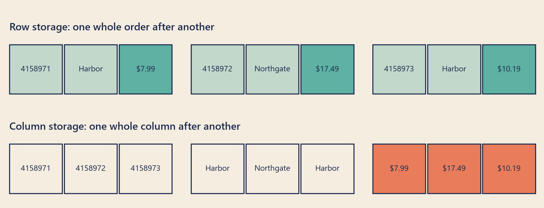
Column storage keeps a table in the same way, and a database built this way is a column store. All the values of one column are stored together: all the order IDs, then all the cities, then all the amounts. To add up net_amount, the reader goes to one shelf and reads only that shelf.
Show the code
sample = steep.q(f""" select order_id, city, net_amount from orders where order_id between {mia_id} and {mia_id +2} order by order_id""")fields = [("order_id", lambda v: str(int(v))), ("city", lambda v: v.title()), ("net_amount", lambda v: bk.fmt_money(float(v)))]row_cells = [(name, show(r[name])) for _, r in sample.iterrows() for name, show in fields]col_cells = [(name, show(r[name])) for name, show in fields for _, r in sample.iterrows()]bk.setup()fig, ax = plt.subplots(figsize=(8, 3.0), layout="constrained")ax.set_axis_off()W, H, GAP =1.0, 0.62, 0.12def strip(cells, y, title, color, reads_all):"""One strip of boxes, in the order the bytes sit on disk. Shaded = read; dark = needed.""" ax.text(0, y + H +0.18, title, fontsize=11, fontweight="semibold", color=bk.INK) x =0for i, (name, text) inenumerate(cells): needed = name =="net_amount"if needed or reads_all: ax.add_patch(Rectangle((x, y), W, H, facecolor=color, alpha=0.75if needed else0.25, edgecolor="none")) ax.add_patch(Rectangle((x, y), W, H, facecolor="none", edgecolor=bk.INK, linewidth=1.1)) ax.text(x + W /2, y + H /2, text, ha="center", va="center", fontsize=8.6, color=bk.INK) x += W + (GAP *3if i in (2, 5) else GAP /3)return xend = strip(row_cells, 1.25, "Row storage: one whole order after another", bk.TEAL, True)strip(col_cells, 0.0, "Column storage: one whole column after another", bk.TOMATO, False)ax.set_xlim(-0.05, end)ax.set_ylim(-0.1, 2.35)plt.show()
Figure 1: Mia’s order and the next two, stored two ways. Shaded boxes are bytes the reader must read to add up net_amount; the darker ones are the values it needs.
Look at Figure 1. In the top strip, the amounts are scattered between IDs and cities, so the reader must pass through every box. In the bottom strip, the amounts sit together, and the reader can skip straight to them.
Column storage has a second gift. Values on one shelf look alike. The status shelf holds three different words, repeated again and again. Values that repeat are easy to compress: to store in fewer bytes than their plain text.
Column storage pays for this somewhere else. To save or read one whole order, a column store must visit every shelf. That is why checkout runs on a row store and analysis runs on a column store. Each shape is built for one kind of work.
The same table, five ways
How big is the difference in practice? Theo stored one week of orders in five ways. He used the week of the drop: 44,772 orders, all 17 columns, as the table stood when Mia pressed “Run”. In this book, 1 KB is a thousand bytes and 1 MB is a million bytes.
Table 1: The same week of orders, stored five ways. Sizes are real file sizes.
Format
Size
Compared with CSV
CSV (text)
7.59 MB
100%
JSON lines (text)
18.62 MB
245%
Parquet, no compression
2.35 MB
31%
Parquet, Snappy
1.67 MB
22%
Parquet, zstd
1.03 MB
14%
CSV (comma-separated values) is a text file with one line per row and commas between the values. Every number is stored as text. A time such as 2026-09-14 08:47:26.933144 takes 26 characters.
JSON lines is also text, with one record per line. But every record repeats every column name, so it is the biggest.
Parquet is a file format for column storage. The three Parquet files differ only in their compression codec: the method used to squeeze the bytes. One uses no codec. One uses Snappy, which is fast but squeezes less. One uses Zstandard, or zstd, which is a little slower but squeezes more.
The zstd Parquet file is about one seventh the size of the CSV file. Bytes not stored are also bytes not read, so a smaller file is a faster file.
Show the code
order = per_col.sort_values("csv_text_bytes").indexfig, ax = bk.figure(8, 5.2)y =range(len(order))ax.barh([i +0.2for i in y], per_col.loc[order, "csv_text_bytes"] / KB, height=0.38, color=bk.TEAL, label="as text (CSV)")ax.barh([i -0.2for i in y], per_col.loc[order, "parquet_zstd_bytes"] / KB, height=0.38, color=bk.TOMATO, label="in Parquet (zstd)")ax.set_yticks(list(y), [f"{c}"for c in order], fontsize=9)ax.grid(axis="x", color=bk.GRID)ax.grid(axis="y", visible=False)ax.set_xlabel("KB for one week of orders")ax.legend(loc="lower right")ax.set_title(f"In Parquet, every column shrinks, and status shrinks from "f"{kb(status_csv)} to {kb(status_pq)}")plt.show()
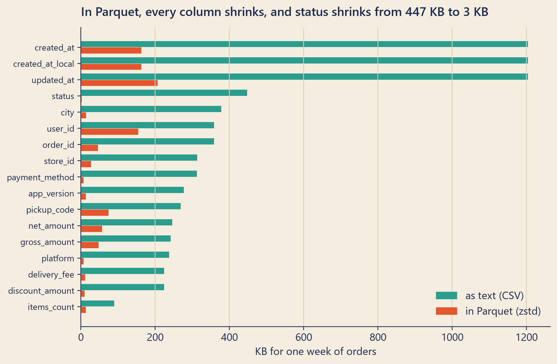
Figure 2: Each column of the same week of orders: as text in the CSV file, and inside the zstd Parquet file.
Figure 2 shows where the bytes go. In Parquet, the three time columns are the biggest: together they hold 52% of the file, because almost every value is different. The status column almost disappears. It needs 3 KB for 44,772 orders, which is less than one bit per order. A bit is the smallest unit of storage: a single 0 or 1. There are eight bits in a byte.
How can a word like “completed” cost less than one bit? Two tricks, and both work best on a column.
Dictionary encoding. The writer makes a short list of the different values, such as 0 = completed, 1 = cancelled and 2 = refunded, and stores each value as its small number. With three values, each number needs only 2 bits.
Run-length encoding. When the same value repeats, the writer stores it once, with a count. That morning, 97% of the week’s orders were completed. In order-ID order, a run of completed was 32 orders long on average. Instead of 32 copies, the file stores one value and the number 32.
A general codec such as zstd then squeezes what is left. In a row store, the statuses sit between times and IDs, so these tricks find much less to work with.
Inside a Parquet file
Apache Parquet is the most common column-storage file format in data lakes. Its cousin Apache ORC (Optimized Row Columnar) grew up with Hive, a tool that runs SQL on files (Chapter 10), and works in a similar way. Here is a Parquet file, from the outside in.
A file holds one or more row groups. A row group is a horizontal slice of the table, for example the first 100,000 rows.
Inside each row group, every column has one column chunk: that column’s values for those rows, stored together. This is the spice rack: one shelf per column, inside each slice.
Each column chunk is cut into pages, the small units that are encoded and compressed.
At the end of the file sits the footer. It lists every row group and every column chunk: where it starts, how big it is, and how it is encoded. For each column chunk, it can also hold statistics: the smallest value, the largest value, and the number of empty values, or nulls.
A reader opens the footer first. The footer tells it where each column chunk starts, so the reader can jump straight to the shelves it needs and skip the others.
Mia found her own order in the lake. It sat in the folder for 14 September and Harbor, in a file of 2,215 orders: one row group, 16 column chunks, and a footer of 3,488 bytes. (The table has 17 columns. The missing one, the city, lives in the folder name, as you will see below.)
The statistics help in a second way. Order numbers count up over time, so each file covers a narrow range of order IDs. That Wednesday, the lake held 456 order files. By their smallest and largest order_id, only the four files of 14 September could contain order 4158971. A reader skips the other 452 files without reading their data. This is called predicate pushdown, or data skipping: the filter is checked against the statistics before the data is read. A predicate is the condition in a WHERE clause, such as order_id = 4158971.
ORC follows the same design under other names. The box “Under the hood” below compares the two formats.
Folders as filters: partitions
Statistics live inside files. Partitions work one level higher, on folders.
Steep’s lake does not keep all orders in one file. It splits them into folders, one for each day, and inside each day, one for each city:
A partition is one of these slices. (Same word, different thing: Chapter 8’s Kafka partitions were slices of a topic. Chapter 10 adds a third meaning.) The columns used for slicing, here dt (the day) and city, are partition columns. The folder name dt=2026-09-14 says that every row inside has that day. The values live in the folder names, not inside the files. This naming style, column=value, comes from Hive (Chapter 10), and it is called Hive-style partitioning. Most tools understand it.
When a query filters on a partition column, the engine reads the folder names and opens only the matching folders. This is partition pruning. Here is the plan that DuckDB, the database engine this book uses, makes for “the total net_amount on 14 September”. (EXPLAIN asks an engine to show its plan without running the query.)
Two lines matter. Projections: net_amount means the reader takes only one column: this is column pruning. Scanning Files shows partition pruning: the reader opens 4 of the 456 files. Reading one column from four files, the engine reads only about 23 KB. The same question on one big CSV file of the same orders would read 118.5 MB.
Choose partition columns with care. A good partition column is one that most queries filter on, such as the day. A bad one has too many values. One folder per user_id would make tens of thousands of tiny folders, which brings us to the next problem.
Too many small files
Every partition is at least one file. That Wednesday, Steep’s lake held 456 order files for 114 days. The average file held 1,613 orders and weighed 61 KB.
On a laptop, that is fine. In a big data system, it is a classic trouble called the small-files problem.
Every file has a fixed cost. A reader must find it, open it and read its footer before it reads any data. Each footer in Steep’s lake is about 3.5 KB, and the footers together make up about 6% of the lake’s bytes. About 36% of each footer is a copy of the table’s schema (its list of columns and their types) that pyarrow, the program that wrote these files, keeps for itself.
Small files compress worse. Each file keeps its own dictionaries, and short columns give the codec less to work with. Theo merged the same 735,637 orders into one file, with the same writer and the same settings. It shrank from 27.8 MB to 19.9 MB: 29% smaller.
Big systems pay per file. Some engines start one task per file. Others pack small files together, but they still list, open and read the footer of each one. The file system of Chapter 10, HDFS, keeps a record of every file in the memory of one central server. Millions of small files make all of this slow.
The cure is compaction: a scheduled job that merges many small files into fewer big ones. Teams also choose coarser partitions when the slices are small, such as one folder per day instead of one per day and city. And they write fewer, bigger files in the first place.
NoteUnder the hood
Bytes read. For a query that needs the set of columns \(S\) and opens the set of files \(F\), a row file reads
Partition pruning makes \(F\) small. Column pruning makes \(S\) small. A row file can only use the first.
The Parquet layout. A file starts with the four bytes PAR1. Then come the column chunks, row group by row group. Then the footer (Parquet calls it the file metadata), then four bytes that give the footer’s length, then PAR1 again. The writer puts the footer last, so it can write the file in one pass. A reader reads the end of the file first. In the footer, each column chunk’s metadata can hold statistics: minimum, maximum and null count. Newer writers can also add a page index, with the minimum and maximum of every page, so a reader can skip single pages.
Encodings. Dictionary encoding stores a column chunk’s distinct values once, in a dictionary page, and stores each value as an index into it. Those indexes use the RLE/bit-packing hybrid: runs of the same value become one count, and the rest are packed with as few bits as the largest index needs, here \(\lceil \log_2 3 \rceil = 2\) bits. If the dictionary grows too big, the writer falls back to plain values. For sorted integers there are also delta encodings, which store the small differences between neighbours. The codec (Snappy, gzip, zstd, LZ4 and others) compresses each page after encoding. In this week of orders, status used 0.45 bits per order.
Row-group size. pyarrow wrote the lake files, one row group each. It also wrote Theo’s merged file. By default, pyarrow puts up to 1,048,576 rows (1024 × 1024) in a row group, so all 735,637 orders fit in one row group. DuckDB, by comparison, starts a new row group every 122,880 rows. The Parquet docs advise large row groups (512 MB to 1 GB) and an HDFS block big enough to hold a whole row group. Steep’s average order file is less than 1/8,000 of 512 MB.
ORC. An ORC file is a list of stripes (big slices, about 64 MB each by default), each with index data, row data and a stripe footer, followed by a file footer and a short postscript. ORC keeps statistics at three levels: the whole file, each stripe, and each group of 10,000 rows inside a stripe (the row index). The statistics hold a count, whether nulls are present, and for most types a minimum and maximum (and a sum for numbers). Both formats can store Bloom filters, a compact structure that answers “is this value possibly here?” with no false “no”. Default settings differ between versions, so check them rather than assume them.
Try it
The bytes-scanned calculator. Pick the columns your query needs and a date filter. The calculator shows how many bytes four storage setups must read for that query. The sizes are real: the CSV text of the 735,637 orders in the lake that Wednesday, and the real Parquet files.
Show the code
bytesCalculator = {const D =JSON.parse(document.getElementById("ch09-calc").textContent);const C = {teal:"#2a9d8f",tealText:"#1f7a6f",tomato:"#e4572e",tomatoText:"#b8401c",ink:"#1d2b4f",paper:"#f4ede0",grid:"#d9cfbd",muted:"#5f6475"};const N = D.days.length;const MONTHS = ["January","February","March","April","May","June","July","August","September","October","November","December"];const asDate = s =>newDate(s +"T00:00:00Z");const dayMonth = s => { const d =asDate(s);return`${d.getUTCDate()}${MONTHS[d.getUTCMonth()]}`; };const range = (from, to) => D.days.map((d, i) => (d >=from&& d <= to ? i :-1)).filter(i => i >=0);const august = D.days.filter(d => d.slice(5,7) ==="08");const FILTERS =newMap([ [`Every day (${dayMonth(D.days[0])} to ${dayMonth(D.days[N -1])})`, [D.days[0], D.days[N -1]]], [`August (${august.length} days)`, [august[0], august[august.length-1]]], [`The week of the drop (${dayMonth(D.week[0])} to ${dayMonth(D.week[1])})`, D.week], [`Mia's first day (${dayMonth(D.oneDay)})`, [D.oneDay, D.oneDay]] ]);const sum = xs => xs.reduce((a, b) => a + b,0);const fmtBytes = b => (b >=1e6?`${(b /1e6).toFixed(1)} MB`:`${Math.max(1,Math.round(b /1e3))} KB`);const colsIn = Inputs.checkbox(D.columns, {value: D.mia,label:"Columns the query needs"});const filterIn = Inputs.radio([...FILTERS.keys()], {value: [...FILTERS.keys()][0],label:"Date filter"});const chartBox = htl.html`<div class="bc-chart"></div>`;const sqlBox = htl.html`<pre class="bc-sql"></pre>`;const noteBox = htl.html`<div class="bc-note" aria-live="polite"></div>`;functioncompute() {const cols = colsIn.value;const [from, to] = FILTERS.get(filterIn.value);const idx =range(from, to);const allCsv =sum(D.columns.map(c =>sum(D.csv[c])));const dayCsv =sum(idx.map(i =>sum(D.columns.map(c => D.csv[c][i]))));const oneCol =sum(cols.map(c => D.oneFile[c])) + (cols.length? D.oneFileOverhead:0);const dayCol =sum(idx.map(i =>sum(cols.map(c => D.pq[c][i])) + (cols.length? D.overhead[i] :0)));const files =sum(idx.map(i => D.files[i]));return {cols,from, to, files,bars: [ {label:"Rows, one big file",sub:"reads every column of every day",bytes: allCsv,color: C.teal}, {label:"Rows, one folder per day",sub:`reads every column of ${idx.length} day${idx.length===1?"":"s"}`,bytes: dayCsv,color: C.teal}, {label:"Columns, one big file",sub:`reads ${cols.length} column${cols.length===1?"":"s"} of every day`,bytes: oneCol,color: C.tomato}, {label:"Columns, one folder per day",sub:`reads ${cols.length} column${cols.length===1?"":"s"} of ${idx.length} day${idx.length===1?"":"s"}, from ${files} files`,bytes: dayCol,color: C.tomato} ]}; }let W =640;// drawing width; follows the page width, so text keeps its real size on phonesfunctionrender() {const r =compute();const max = r.bars[0].bytes;const FS = W <480?13:14, LEFT =8, BAR =18, ROW =58, H = r.bars.length* ROW +6;const shapes = r.bars.flatMap((b, k) => {const y =4+ k * ROW;const w =Math.max(2, (W - LEFT -8) * b.bytes/ max);const share = b.bytes/ max;return [ htl.svg`<text x="${LEFT}" y="${y +13}" font-size="${FS}" font-weight="600" fill="${C.ink}">${b.label}</text>`, htl.svg`<text x="${W -4}" y="${y +13}" font-size="${FS}" font-weight="600" text-anchor="end" fill="${C.ink}">${fmtBytes(b.bytes)}${k ?` · ${share >=0.1?Math.round(100* share) : (100* share).toFixed(share >=0.001?1:2)}%`:""}</text>`, htl.svg`<rect x="${LEFT}" y="${y +20}" width="${W - LEFT -8}" height="${BAR}" fill="${C.grid}" fill-opacity="0.45" rx="3"/>`, htl.svg`<rect x="${LEFT}" y="${y +20}" width="${w}" height="${BAR}" fill="${b.color}" rx="3"/>`, htl.svg`<text x="${LEFT}" y="${y +52}" font-size="12" fill="${C.muted}">${b.sub}</text>` ]; }); chartBox.replaceChildren(htl.svg`<svg viewBox="0 0 ${W}${H}" width="100%" role="img" aria-label="${r.bars.map(b =>`${b.label}: ${fmtBytes(b.bytes)}`).join("; ")}" style="max-width:${W}px;font-family:Inter,system-ui,sans-serif">${shapes}</svg>`);const list = r.cols.length? r.cols.join(", ") :"(no columns)"; sqlBox.textContent=`SELECT ${list}\nFROM ods_orders\nWHERE dt BETWEEN DATE '${r.from}' AND DATE '${r.to}'`;const best = r.bars[3].bytes, worst = r.bars[0].bytes;let note = r.cols.length===0?"Pick at least one column.":`The column store with day folders reads ${fmtBytes(best)}: about 1/${Math.max(1,Math.round(worst / best)).toLocaleString("en-US")} of the big row file.`;if (r.cols.length&& r.bars[3].bytes> r.bars[2].bytes) { note +=" Here the day folders read more than one big file: every small file brings its own footer and dictionaries."; } noteBox.textContent= note; }const button = (label, action) => {const b = htl.html`<button type="button" class="bc-btn">${label}</button>`; b.addEventListener("click", () => { action();render(); });return b; };const setCols = cols => { colsIn.value= D.columns.filter(c => cols.includes(c));// keep the table's column order colsIn.dispatchEvent(newEvent("input", {bubbles:true})); }; colsIn.addEventListener("input", render); filterIn.addEventListener("input", render);render();const resizer =newResizeObserver(() => {const next =Math.max(300,Math.min(640,Math.round(chartBox.clientWidth) ||640));if (next !== W) { W = next;render(); } }); resizer.observe(chartBox); invalidation.then(() => resizer.disconnect());const style =document.createElement("style"); style.textContent=` .bc-wrap { font-family: Inter, system-ui, sans-serif; color: ${C.ink}; } .bc-wrap form { max-width: 100%; } .bc-wrap label { font-size: 0.82rem; } .bc-buttons { display: flex; flex-wrap: wrap; gap: 0.4rem; margin: 0.2rem 0 0.7rem; } .bc-btn { font: 600 0.85rem Inter, system-ui, sans-serif; color: ${C.paper}; background: ${C.ink}; border: 0; border-radius: 5px; padding: 0.45rem 0.8rem; cursor: pointer; } .bc-btn:hover { background: ${C.tealText}; } .bc-btn:focus-visible { outline: 3px solid #f2b134; outline-offset: 2px; } .bc-sql { font-size: 0.76rem; white-space: pre-wrap; word-break: break-word; margin: 0.6rem 0; background: rgba(29, 43, 79, 0.06); padding: 0.5rem 0.7rem; border-radius: 5px; } .bc-note { font-size: 0.85rem; min-height: 2.6em; margin-top: 0.3rem; }`;return htl.html`<div class="bc-wrap">${style} <div class="bc-buttons">${button("Mia's question", () =>setCols(D.mia))}${button("One column", () =>setCols(["net_amount"]))}${button("Every column (SELECT *)", () =>setCols(D.columns))} </div>${colsIn}${filterIn}${sqlBox}${chartBox}${noteBox} </div>`;}
Things to try:
Press “Mia’s question” with every day. The big row file reads 118.5 MB. One big column file reads 4.5 MB, about 4% of that.
Press “One column” and choose Mia’s first day. The column store with day folders reads about 23 KB, most of it the four footers.
Go back to every day. With day folders, the column store now reads more than one big column file: the small-files problem, in bytes.
The calculator counts bytes only. Real engines also use statistics, caches and indexes, and real row stores keep binary rows, smaller than CSV lines. The lake files hold each order’s status as of the end of October, which barely changes the sizes. The direction of every comparison stays the same.
Common traps
Running analysis on production. Even a query that only reads takes processors, memory and disk away from customers. Use a read replica, the lake or the warehouse.
SELECT * on a column store. It throws away the main advantage. Name the columns you need.
Filtering on the wrong column. In Steep’s lake, WHERE dt = '2026-09-14' prunes folders. A filter on the date part of created_at_local asks the same question, but created_at_local is not a partition column. The engine must at least open every file to check it.
Partitioning by a column with too many values. Tens of thousands of tiny folders give you the small-files problem.
An index for every report. Each index slows down the writes that touch it: every new order, and every change to its columns. Reports belong in the lake, not in more indexes on production.
TipAudit Instinct · Extracts, not queries on production
In an IT audit, IT general controls (ITGCs) are the basic controls over a company’s systems: who can access them, how changes are made, and how they are run. One habit follows: auditors do not run heavy queries on the live system. They ask for an extract, a copy of the data taken at a set time. It does not slow down the business, and it does not change while the auditor works.
A second control is segregation of duties: the people and systems that report on operations are kept apart from the operations themselves. A report should not be able to stop the cash register.
Mia’s morning was a small ITGC finding: an analyst had read access to production. Theo fixed the control, not the person. That afternoon he removed her access to the orders database and pointed her to the lake.
NoteInterview Corner
Q1. Why is columnar storage faster for analytics?
NoteA short answer
Analytical queries read a few columns of many rows. A column store reads only those columns, and the values of one column look alike, so they compress very well (dictionary and run-length encoding, then a codec). Fewer bytes from disk means less time. Formats such as Parquet and ORC also keep minimum and maximum values per chunk, so the reader can skip chunks that cannot match the filter. Engines can also process a column in batches, which suits modern processors. The price: writing or reading one whole row touches every column, so OLTP systems stay with rows.
Q2. ORC or Parquet?
NoteA short answer
Both are open, columnar, compressed and self-describing, with statistics for data skipping, and both can store Bloom filters. ORC grew up in Hive: it uses large stripes, keeps statistics for every 10,000 rows, and is the format behind Hive’s transactional (ACID) tables. Parquet uses row groups, column chunks and pages, can keep statistics for every page, and handles nested data well. It has the widest support across engines: it is Spark’s default data source and the usual file format under table formats such as Iceberg and Delta Lake. In practice, choose the one your engines support best. Today that is usually Parquet, unless the stack is built around Hive.
Q3. What is the small-files problem, and how do you fix it?
NoteA short answer
Too many files that are much smaller than the storage block or the recommended row-group size. Each file costs a lookup, an open and a footer read, and sometimes a task of its own. In HDFS (Chapter 10), one central server keeps a record of every file in its memory. Small files also compress worse. Causes: too many partitions, streaming jobs that write often, and too many parallel writers.
Fixes when writing: compact files on a schedule. Control how many tasks write each partition, so that each partition gets a few big files. Use coarser partitions. Or use a table format with built-in compaction (Chapter 11).
Fixes when reading: let the engine pack many small files into one task. This saves tasks, but not the cost of opening every file. Chapter 10’s “Under the hood” names the Hive and Spark settings for both.
Q4. Why does MySQL’s InnoDB use B+ trees, and not B-trees, binary trees or hash tables?
NoteA short answer
Disks are read in pages, and InnoDB keeps whole pages in memory, so the goal is to find a row in as few page reads as possible. In a B+ tree, each inner page has hundreds of children, so even millions of rows need only three or four levels. Records live only in the leaves, so the upper pages hold keys alone and fit more of them: the tree is shorter. The leaves are linked in order, so range scans and ORDER BY walk along them, and every lookup takes the same number of steps. A binary tree, even a balanced one such as a red-black tree, is far deeper (about 23 levels for 4.2 million keys), and each level can cost a page read. A hash table finds an exact key fast, but it keeps no order, so it cannot serve ranges, sorting or a leftmost prefix. (InnoDB can also add an adaptive hash index on top of its B-trees for frequent exact lookups; since MySQL 8.4 it is off by default.)
Q5. What is the difference between a clustered and a secondary index? What is 回表?
NoteA short answer
In InnoDB, the clustered index is the table: a B+ tree on the primary key whose leaf pages hold the whole rows, so there is exactly one per table. (Without a primary key, InnoDB uses the first unique index on columns that are never NULL, or else a hidden row ID.) A secondary index stores its own columns plus the primary key. A lookup through it finds the primary key first, then searches the clustered index for the row: that second search is 回表, “back to the table”. A short primary key keeps every secondary index small.
Q6. What is a covering index?
NoteA short answer
An index that holds every column a query needs, so the query is answered from the index alone, with no trip back to the table. Example: with an index on (store_id, created_at), counting one store’s orders in one hour reads only the index. In InnoDB, every secondary index also carries the primary key, so a query for order_id can be covered too. In MySQL, EXPLAIN shows Using index in its Extra column. Do not confuse it with Using index condition, which means the index filtered rows first but the rows were still read (see Q7).
Q7. Explain the leftmost-prefix rule with an example.
NoteA short answer
A composite index on (a, b, c) is sorted by a, then b, then c. It can narrow a search on a; on a and b; and on a, b and c. It cannot narrow a search on b alone, c alone, or b and c, because those values are scattered across the whole index. Example: an index on (store_id, created_at, status) helps WHERE store_id = 'HBR-01' AND created_at >= …, but not WHERE created_at >= … on its own. After a range condition such as >=, later columns (here status) no longer narrow the search; they can only filter. The order of the conditions in WHERE does not matter. With WHERE a = 1 AND c = 3, only a narrows the search, and MySQL checks c inside the index before going back to the table. This is index condition pushdown (索引下推); EXPLAIN shows Using index condition. MySQL 8 can sometimes use a skip scan, but only when the query needs no column outside the index and the first column has few values.
Q8. When does a query stop using an index?
NoteA short answer
Often, but not always, since optimisers differ: when the column is wrapped in a function or an expression; when a LIKE pattern starts with a wildcard; when types differ, such as a text column compared with a number; when the leftmost column of a composite index is missing; with OR across different columns (unless the optimiser merges two indexes); and when the query touches a large share of the table, so a full scan is cheaper. Check with EXPLAIN instead of guessing.
Reported change: −12.0% orders, the week of 7 September compared with the week before (CEO dashboard).
Explained so far: 0 of the 12 points. About 7 of them sit between the orders database and the dashboard (Clue 1).
Suspects: the iOS app, version 3.2.0 (Chapter 6): the main suspect, not proved. The service that writes app events to Kafka (Chapter 8): a minor suspect.
Ruled out: the matcha menu (Chapter 4), Kafka (Chapter 8), and now storage (Chapter 9).
Open questions: Do the jobs between the lake and the dashboard lose anything? Was there a gap before September? (Chapter 10.) What exactly broke, and how many points does it explain? (Chapter 15.)
New evidence: the lake holds 735,637 orders up to 22 September, the same number as the database. Its copy of Monday 14 September’s events holds 51,927 events, the same number as Kafka’s dump. Order A1024 sits in dt=2026-09-14/city=harbor. The lake holds four events from Mia’s phone that morning, and no order_completed. The lake stored exactly what it was given. A new habit: big questions go to the lake, never to production.
Recap
Row storage keeps each record together, and a B+ tree index finds one row in a few page reads: right for saving and finding single orders (OLTP). Column storage keeps each column together: right for reading a few columns of many rows (OLAP).
Columnar formats such as Parquet and ORC compress well and carry statistics, so a reader can skip columns, files and chunks. Partition folders let it skip whole days.
Partitions have a price. Too many small files cost more than they save, so compact them.
Rudolf Bayer and Edward McCreight, “Organization and maintenance of large ordered indexes”, Acta Informatica 1(3), 1972. doi:10.1007/BF00288683. The paper that introduced the B-tree.
Douglas Comer, “The ubiquitous B-tree”, ACM Computing Surveys 11(2), 1979. doi:10.1145/356770.356776. A readable survey, including the B+ tree.
Patrick O’Neil, Edward Cheng, Dieter Gawlick and Elizabeth O’Neil, “The log-structured merge-tree (LSM-tree)”, Acta Informatica 33(4), 1996. doi:10.1007/s002360050048.
Daniel J. Abadi, Samuel R. Madden and Nabil Hachem, “Column-stores vs. row-stores: how different are they really?”, Proceedings of the 2008 ACM SIGMOD International Conference on Management of Data. doi:10.1145/1376616.1376712. A careful study of why column stores are fast.