On Friday morning, a slide was waiting on the big screen in the meeting room. Marketing had sent it to Dana the evening before. Its title said: New competitor in Northgate: orders are collapsing.
Under the title stood fourteen bars, one for each day of the last two weeks, as the dashboard counted them. The bars of the first week were tall. The bars of the second week were short. The bar for Monday 7 September was tiny.
Dana came in with her laptop and sat down. “I owe the board a short note today,” she said. “One chart about the drop. One chart that I can defend when somebody asks a hard question. Marketing wants me to send this one.”
Mia looked at the slide for a while. Then she pointed at the bottom of it.
“The axis starts at 5,000, not at zero.”
“Does that matter? Marketing checked the numbers.”
“The numbers are right,” said Mia. “Every bar has the correct height above 5,000. But nobody looks at the numbers on the axis. People look at the bars. And the bars say that orders fell by almost half.”
Theo had come in with his tea and was standing at the back. “Every chart is a choice,” he said. “This one chose drama.” Nobody laughed, but Dana smiled.
“Then draw me the honest one,” Dana said. “Before noon, please.”
Mia opened her notebook. When she reviewed a report as an auditor, she always asked three questions, and she wrote them down again now: What is the question? Does the picture match the numbers? What is missing?
ImportantThe big idea
A chart is an argument. Choose the picture that answers the question, and make the honest reading the easiest one to see.
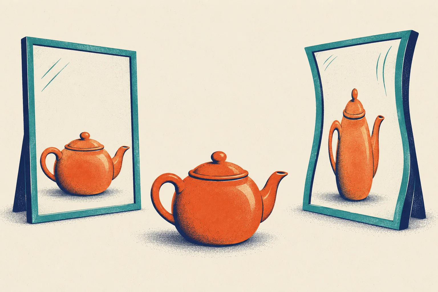
Look at the picture. One teapot, two mirrors. The flat mirror shows the pot as it is. The curved mirror shows the same pot, tall and thin. Nothing in the curved mirror is invented: the lid, the spout and the handle are all there. Only the shape is stretched. Most misleading charts are curved mirrors. They do not invent data. The data is real; the drawing bends it.
A chart answers a question
Before you draw anything, write down the question that the chart must answer. The question chooses the chart, not the other way round. A few questions come up again and again:
Your question
A good first chart
A Steep example
How did it change over time?
A line chart
Orders per day
How do a few groups compare?
A bar chart, sorted
The change in orders, by city
What share is each part of the whole?
A stacked bar (a pie only with two or three parts)
Orders by platform
How are the values spread out?
A histogram
Order value (Chapter 2)
Do two numbers move together?
A scatter plot
Rain and orders (Chapter 16)
Dana’s question was simple: did orders really fall, and by how much? Marketing’s slide answered a different question: how different do the two weeks look? With a cut axis, the answer is “very”.
The bar that started at 5,000
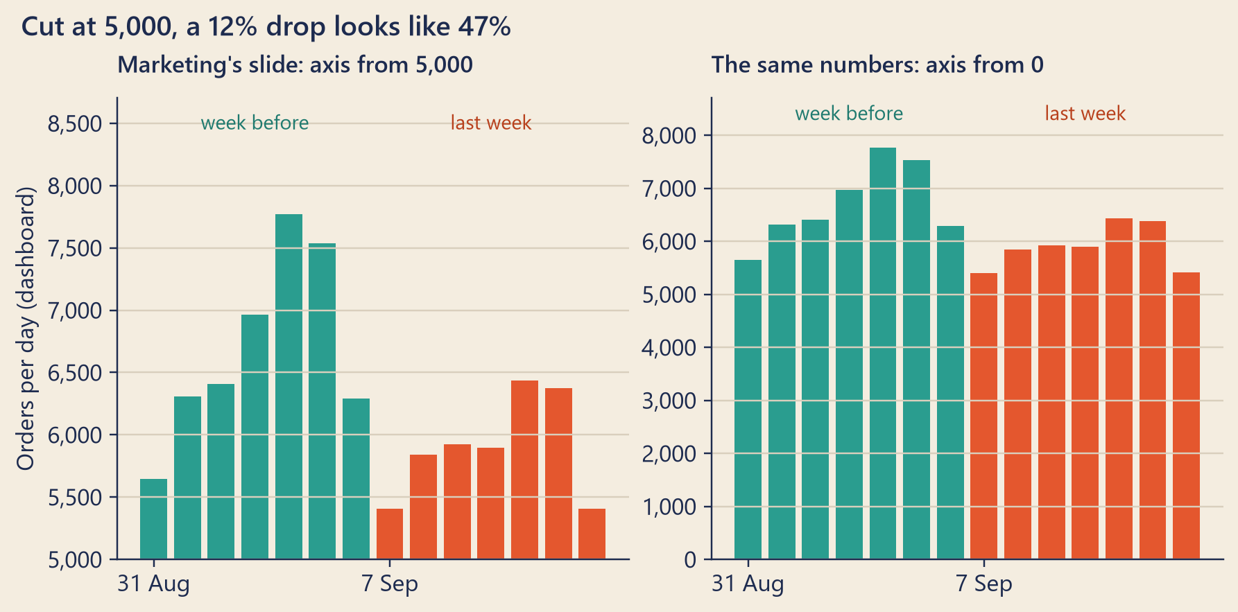
Here is marketing’s slide again, next to the same fourteen numbers drawn with the axis starting at zero.
Show the code
bk.setup()colors = [bk.TEAL if d <= W1_END else bk.TOMATO for d in two.day]top = two.dashboard.max() *1.12fig, axes = plt.subplots(1, 2, figsize=(8, 3.9), layout="constrained")for ax, base, title in [(axes[0], SLIDE_BASE, f"Marketing's slide: axis from {n(SLIDE_BASE)}"), (axes[1], 0, "The same numbers: axis from 0")]: ax.bar(two.day, two.dashboard - base, bottom=base, color=colors, width=0.8) ax.set_ylim(base, top) ax.set_title(title, fontsize=11) thousands(ax) mondays(ax, two.day.min(), two.day.max())for start, label, color in [(W1_START, "week before", bk.TEAL_TEXT), (W2_START, "last week", bk.TOMATO_TEXT)]: ax.text(start + pd.Timedelta(days=3), top *0.985, label, color=color, ha="center", va="top", fontsize=9.5)axes[0].set_ylabel("Orders per day (dashboard)")fig.suptitle(f"Cut at {n(SLIDE_BASE)}, a {bk.fmt_pct(-reported, 0)} drop looks like "f"{bk.fmt_pct(-seen_change, 0)}", x=0.01, ha="left", fontsize=13, fontweight="semibold", color=bk.INK)plt.show()
Figure 1: The dashboard’s orders for each day of the two weeks. Left: marketing’s slide, with the y-axis starting at 5,000. Right: the same numbers, with the y-axis starting at zero.
Both charts use the same numbers. On average, the dashboard counted 6,703 orders a day in the week before and 5,898 last week: a change of −12.0%. But on the slide, a bar shows only the part above 5,000. That part shrank from 1,703 to 898, so the bars look 47% shorter. The picture shows a change about 4 times bigger than the data. Look at single days, and it gets worse. On the slide, the bar for Monday 7 September is only 15% as tall as the bar for Friday 4 September. In the data, that Monday had 70% as many orders as that Friday.
Why does this fool people? Because a bar is a length. Your eye reads the length of each bar and compares the lengths, and it does this before you read a single number on the axis. A bar that starts at 5,000 is not the number. It is the number minus 5,000. So bars must start at zero. The same rule holds for anything that shows a quantity by its size: areas, stacked bars and bubbles.
A truncated axis is an axis that does not start at zero. For bars it is almost always wrong. For line charts it can be fine. A line shows a value by its position, not by its length, and the eye reads its shape: up, down, flat. When the question is about change, it can help to zoom in on the range where the data lives. Two conditions: label the axis clearly, and do not let the zoom turn small noise into a dramatic story. A good test: would a reader who ignores the axis numbers come away with the right idea? If not, zoom out.
NoteUnder the hood
The lie factor. Edward Tufte gave a name to how much a chart exaggerates:
\[\text{lie factor} = \frac{\text{size of the change shown in the picture}}{\text{size of the change in the data}},\]
where the size of a change from \(a\) to \(b\) is \(|b - a| / a\). An honest chart has a lie factor close to 1.
For bars cut at a base \(c\), the eye compares \(b - c\) with \(a - c\), so the picture’s change is
\[\frac{(b - c) - (a - c)}{a - c} = \frac{b - a}{a - c},\]
larger than the real \(\frac{b - a}{a}\) by a factor of \(\frac{a}{a - c}\). With \(a\) = 6,703 and \(c\) = 5,000, that factor is 3.9, which is the lie factor above. The closer the cut sits to the data, the bigger the lie.
Position beats angle. William Cleveland and Robert McGill tested how well people read charts. People compared values more accurately when the values sat as positions on a shared scale, such as dots or the ends of bars on one axis. They did worse when they had to compare angles, as in a pie chart. That is why a sorted bar chart or a dot chart usually beats a pie.
Is it Northgate?
The slide’s title made a second claim: the drop came from a new competitor in Northgate. A chart of all of Steep cannot test that. A chart that compares the cities can. If a competitor in Northgate were taking customers away, Northgate should fall more than the other cities.
Mia also wanted to separate the two sources. She knew from Chapter 1 that the dashboard and the database disagree. So for each city she drew two bars: the change in the database’s completed orders, and the change on the dashboard.
Show the code
fig, ax = bk.figure(8, 3.9)ax.grid(axis="y", visible=False)ax.grid(axis="x", color=bk.GRID)ax.set_axisbelow(True)cities =list(city_change.index)height =0.36for i, city inenumerate(cities):for offset, source, color in [(-height /2, "database", bk.INK), (height /2, "dashboard", bk.TOMATO)]: value =100* city_change.loc[city, source] ax.barh(i + offset, value, height=height *0.92, color=color) label =f"{bk.fmt_pct(value /100, 1)}"if i ==0: label =f"{source}{label}" ax.text(value -0.25, i + offset, label, ha="right", va="center", fontsize=9, color=bk.INK if source =="database"else bk.TOMATO_TEXT)ax.set_yticks(range(len(cities)), cities)ax.invert_yaxis()ax.axvline(0, color=bk.INK, lw=0.9)ax.set_xlim(100* city_change.dashboard.min() *1.55, 0.6)ax.xaxis.set_major_locator(mticker.MultipleLocator(5))ax.xaxis.set_major_formatter(mticker.FuncFormatter(lambda v, _: f"{v:.0f}%".replace("-", "−")))ax.set_xlabel("Change, week before → last week")ax.tick_params(axis="y", length=0)ax.set_title("In every city, the dashboard fell more than the database")plt.show()
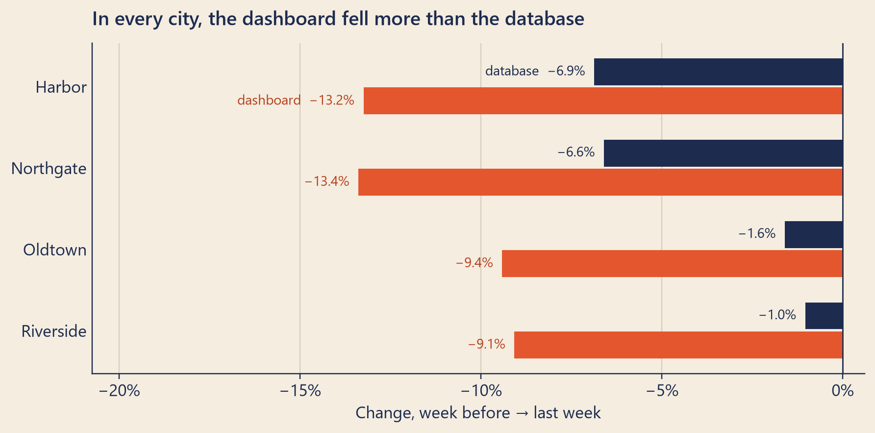
Figure 2: The change in orders from the week before to last week, by city. Dark blue: completed orders in the database. Tomato: the dashboard’s count. Cities are sorted by the database’s change.
Read the dark blue bars first: the database, the record of real money. Harbor fell 6.9% and Northgate 6.6%. Northgate did not fall more than Harbor, and nobody says that Harbor has a new competitor. Oldtown and Riverside fell less. (Chapter 16 asks why the two big cities fell more.) Now read the tomato bars. In every city, the dashboard fell much further than the database.
So the chart says something different from the slide. There is no sign of a drop that belongs to Northgate alone. There is a sign of a measurement problem that belongs to every city.
Three small choices make this chart easy to read:
Sorting. The cities are sorted by the database’s change, so the eye walks from the biggest fall to the smallest without jumping back and forth. Here the alphabet happens to give the same order; with more cities it rarely does. The order you choose decides which city the reader sees first.
Direct labels. Each bar carries its own number, and the first pair names the two sources. A legend, the little key in a corner that matches colours to names, makes the reader look away from the data and back again. Write the name next to the line or bar instead.
A title that states the finding. “Orders by city, week over week” names the topic. “In every city, the dashboard fell more than the database” tells the reader what to see. The reader can then check the claim against the picture.
Big cities, small cities, one scale
Harbor makes about 2,644 completed orders a day. Riverside makes about 936. Put both on one axis, and the same 10% change moves Riverside’s line only about a third as far as Harbor’s. This is a common problem: the same metric, on very different scales.
Mia’s answer was to change the question into one that has the same scale everywhere: for every 100 completed orders in the database, how many did the dashboard count? Then she drew one small chart for each city, all with the same axes. A set of small charts that share their axes is called small multiples. Because the axes match, the eye can compare the shapes from one chart to the next.
Show the code
fig, axes = plt.subplots(2, 2, figsize=(8, 5.2), sharex=True, sharey=True, layout="constrained")for ax, city inzip(axes.flat, sorted(view.city.unique(), key=lambda c: -daily_size[CITY[c]])): part = view[view.city == city] ax.plot(part.day, part.per100, color=bk.TOMATO, lw=2) ax.axhline(100, color=bk.MUTED, lw=1) ax.axvline(SPLIT, color=bk.INK, ls="--", lw=1) ax.set_title(f"{CITY[city]} · about {n(daily_size[CITY[city]])} orders a day", fontsize=10.5) mondays(ax, VIEW_START, VIEW_END, every=2)axes[0, 0].text(SPLIT, 81, " 7 Sep", fontsize=9, color=bk.INK, va="bottom")for ax in axes[:, 0]: ax.set_ylabel("Per 100 in database")axes[0, 0].set_ylim(80, 108)fig.suptitle("In every city, the dashboard began to miss orders on 7 September", x=0.01, ha="left", fontsize=13, fontweight="semibold", color=bk.INK)plt.show()
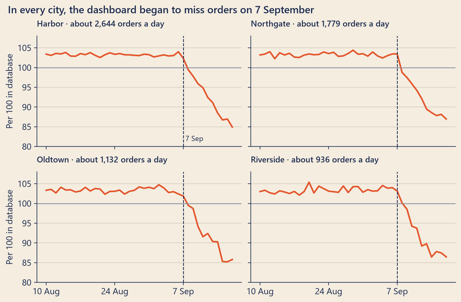
Figure 3: Dashboard orders for every 100 completed orders in the database, day by day, in each city. The dashed line marks 7 September.
Four cities of very different sizes, and one shape. Before 7 September, the dashboard counted between 102 and 105 orders for every 100 in the database, on every day and in every city. (It counts a little more than finance because the app reports an order at payment, before anyone knows whether it will be cancelled or refunded: Chapter 1.) From 7 September, the line slides down. By 17 September, it was between 85 and 87, in all four cities.
There are other answers to the same problem. You can show each city’s percent change, as in Figure 2. Or you can set each city’s starting value to 100 and draw the change from there. A series scaled this way is called an index. Small multiples can also give each chart its own y-axis, if the question is about shape rather than size. If you do that, say so in the caption, because readers assume shared axes.
Two axes, two stories
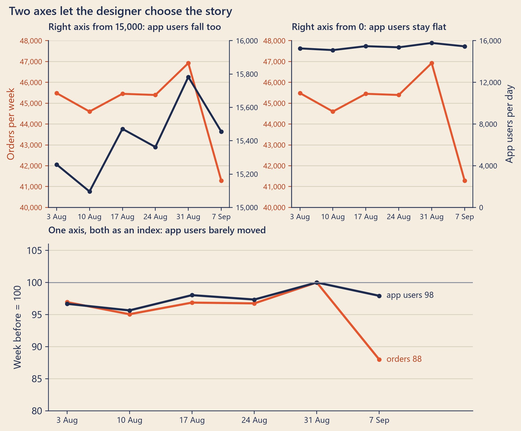
Marketing’s deck had a second chart with two lines. One line was the dashboard’s orders per week. The other was the number of app users: people who opened the app on a day, on average per day. An app user is not the same as an active customer, a person who placed at least one order, counted in the database (Chapter 6 counts those). Orders are counted per week and app users per day, so each line got its own y-axis, one on each side. Both lines fell together in the last week. The slide’s message: customers are leaving.
A chart with two y-axes is a dual-axis chart. It has a hidden problem. Each axis can be stretched or squeezed on its own, so the designer decides where the lines sit, how steep they look, and where they cross. Mia drew the same data twice, changing only where the right axis starts.
Show the code
labels = [f"{w.day}{w.strftime('%b')}"for w in weekly.week]x = np.arange(len(weekly))fig, axes = plt.subplot_mosaic([["A", "B"], ["C", "C"]], figsize=(8, 6.6), layout="constrained")for key, users_bottom, title in [("A", USERS_ZOOM, f"Right axis from {n(USERS_ZOOM)}: app users fall too"), ("B", 0, "Right axis from 0: app users stay flat")]: ax = axes[key] ax.plot(x, weekly.orders, color=bk.TOMATO, lw=2.2, marker="o", ms=4) ax.set_ylim(*ORDERS_AXIS) thousands(ax) ax.tick_params(axis="y", colors=bk.TOMATO_TEXT, labelsize=8.5) right = ax.twinx() right.plot(x, weekly.users, color=bk.INK, lw=2.2, marker="o", ms=4) right.set_ylim(users_bottom, USERS_TOP) right.spines["right"].set_visible(True) right.grid(False) right.tick_params(axis="y", colors=bk.INK, labelsize=8.5) right.yaxis.set_major_formatter(mticker.FuncFormatter(lambda v, _: f"{v:,.0f}")) right.yaxis.set_major_locator(mticker.MaxNLocator(5)) ax.right_ax = right ax.set_xticks(x, labels, fontsize=8.5) ax.set_title(title, fontsize=10.5)axes["A"].set_ylabel("Orders per week", color=bk.TOMATO_TEXT)axes["B"].right_ax.set_ylabel("App users per day", color=bk.INK)ax = axes["C"]ax.plot(x, weekly.orders_index, color=bk.TOMATO, lw=2.4, marker="o", ms=4)ax.plot(x, weekly.users_index, color=bk.INK, lw=2.4, marker="o", ms=4)ax.axhline(100, color=bk.MUTED, lw=1)ax.set_xticks(x, labels, fontsize=9)ax.set_xlim(-0.3, len(x) -0.3)ax.set_ylim(80, 106)ax.set_ylabel("Week before = 100")ax.text(x[-1] +0.08, weekly.orders_index.iloc[-1], f" orders {weekly.orders_index.iloc[-1]:.0f}", color=bk.TOMATO_TEXT, va="center", fontsize=9.5)ax.text(x[-1] +0.08, weekly.users_index.iloc[-1], f" app users {weekly.users_index.iloc[-1]:.0f}", color=bk.INK, va="center", fontsize=9.5)ax.set_xlim(-0.3, len(x) +0.5)ax.set_title("One axis, both as an index: app users barely moved", fontsize=10.5)fig.suptitle("Two axes let the designer choose the story", x=0.01, ha="left", fontsize=13, fontweight="semibold", color=bk.INK)plt.show()
Figure 4: Top: the dashboard’s orders per week (tomato, left axis) and app users per day (dark blue, right axis), drawn twice with different right axes. Bottom: both as an index, with the week before set to 100, on one axis.
The top two charts use the same 12 numbers. On the left, the right axis runs from 15,000, and app users seem to fall with orders. On the right, it runs from zero, and app users look flat. Neither chart has a wrong number in it. They tell opposite stories because of one setting that most readers never check.
The honest version uses one axis. Mia turned both lines into an index: each week’s value divided by the value of the week before the drop, times 100. Now both lines share one unit, “percent of the week before”, and one axis. App users changed by −2.1%. The dashboard’s orders changed by −12.0%. People kept opening the app. Fewer orders reached the dashboard.
An index depends on its base week. Here the base, the week before the drop, was the highest of the six weeks for both lines, so every other week looks low next to it. Always say which week you chose. (Chapter 16 asks why that week was so high.)
So the rule is short: if two lines measure the same thing, put them on one axis. If they measure different things, make them the same thing first (an index, or a percent change), or draw two charts, one above the other, with the same x-axis.
Colour, labels and the chart for the board
By eleven o’clock, Mia had one chart left to draw: the one for the board. She asked her three questions once more.
What is the question? Did orders really fall, and by how much? So the chart needs both counts: the dashboard’s, and the database’s.
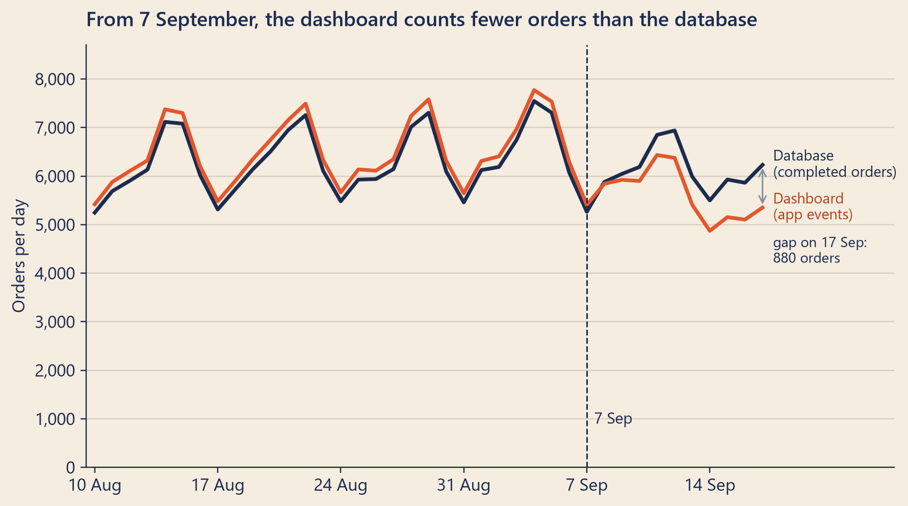
Does the picture match the numbers? Both lines count orders, so they share one axis. Mia started the axis at zero. A line may zoom in, but for the board she wanted no doubt: the gap is big enough to see from zero, and nobody can say she stretched it.
What is missing? The date when things changed, written on the chart, and plain labels at the end of each line instead of a legend.
She also chose the colours with care. In this book, teal and tomato mean “before” and “after”, or “version A” and “version B”. This chart has no before and after; it has a record and a suspect. So the database, the record of money, is dark blue. The dashboard, the line under suspicion, is tomato. One strong colour tells the eye where to look.
Figure 5: Orders per day from 10 August to 17 September. Dark blue: completed orders in the orders database (finance’s count). Tomato: the CEO dashboard, which counts order_completed events from the app.
Read it from left to right. For four weeks, the two lines move together, up on Fridays and Saturdays and down on Mondays, with the dashboard a little above the database: about 103 for every 100. Then, on 7 September, they part. On Tuesday 8 September, the dashboard falls below the database for the first time, by 36 orders. After that the gap widens on almost every day. On Thursday 17 September, the database recorded 6,231 completed orders and the dashboard showed 5,351: 880 orders, or 14%, missing. (The database line uses final statuses; see Chapter 1.)
Dana looked at it for a long time.
“So the orders did fall,” she said. “But not as much as my screen says. And the difference started on one day.”
“Yes. In the database this morning, last week was −4.9% against the week before. On the dashboard, −12.0%.”
“Do you know what happened on 7 September?”
“Not yet,” said Mia. “But I know where to look. On Wednesday, my SQL put almost all of the gap on iOS. This afternoon I want to follow iPhone customers through the app, step by step.”
Dana pasted the chart into her note to the board, under one sentence: Our dashboard has been undercounting orders since 7 September; we are finding out why. Then she forwarded marketing’s slide to Mia with three words: Please explain axes.
Try it
Bend the mirror yourself. Three real Steep charts. Change one setting at a time, and watch the story change while the numbers stay the same.
{const weeks = chartFacts.weekly;const ref = weeks[weeks.length-2];const narrow = chartWidth <520;// on a phone, tilt the week labels so they do not overlapconst common = {width: chartWidth,height:260,marginLeft:56,marginRight:60,marginBottom: narrow ?52:36,style: {background:"transparent",fontSize:"11px"},x: {type:"point",domain: weeks.map(d => d.week),label:null,padding:0.3,tickRotate: narrow ?-40:0}};if (dualMode !=="Two axes") {const rows = weeks.flatMap(d => [ {week: d.week,series:"orders",value:100* d.orders/ ref.orders}, {week: d.week,series:"app users",value:100* d.users/ ref.users}]);const lastWeek = rows.slice(-2);return Plot.plot({...common,y: {domain: [80,106],label:"↑ Week before = 100",grid:true},marks: [ Plot.ruleY([100], {stroke: chartColors.muted}), Plot.line(rows, {x:"week",y:"value",z:"series",strokeWidth:2.4,stroke: d => (d.series==="orders"? chartColors.tomato: chartColors.ink)}), Plot.dot(rows, {x:"week",y:"value",r:3,fill: d => (d.series==="orders"? chartColors.tomato: chartColors.ink)}), Plot.text(lastWeek, {x:"week",y:"value",dx:8,textAnchor:"start",text: d =>`${d.series}${d.value.toFixed(0)}`,fill: d => (d.series==="orders"? chartColors.tomatoText: chartColors.ink)}) ]}); }const [L0, L1] = chartFacts.ordersAxis;const R0 = usersBottom, R1 = chartFacts.usersTop;const toLeft = u => L0 + (u - R0) / (R1 - R0) * (L1 - L0);const rightTicks = d3.ticks(R0, R1,4);const rightLabel =newMap(rightTicks.map(t => [toLeft(t), t.toLocaleString("en-US")]));return Plot.plot({...common,y: {domain: [L0, L1],label:null,tickFormat: d => d.toLocaleString("en-US")},marks: [ Plot.line(weeks, {x:"week",y:"orders",stroke: chartColors.tomato,strokeWidth:2.4}), Plot.dot(weeks, {x:"week",y:"orders",fill: chartColors.tomato,r:3}), Plot.line(weeks, {x:"week",y: d =>toLeft(d.users),stroke: chartColors.ink,strokeWidth:2.4}), Plot.dot(weeks, {x:"week",y: d =>toLeft(d.users),fill: chartColors.ink,r:3}), Plot.axisY({anchor:"left",color: chartColors.tomatoText,label:"↑ Orders per week"}), Plot.axisY([...rightLabel.keys()], {anchor:"right",color: chartColors.ink,tickFormat: d => rightLabel.get(d),label:"App users per day ↑"}) ]});}
3 · Sort and label. The change in orders by city, from the week before to last week.
Show the code
viewof citySort = Inputs.radio(["A to Z","By the dashboard's change"], {value:"A to Z",label:"Sort cities"})
Show the code
viewof cityNames = Inputs.radio(["A legend","Labels on the bars"], {value:"A legend",label:"Name the bars with"})
Show the code
{const rows = chartFacts.cities.map(d => ({...d,value:100* d.change}));const dash =newMap(rows.filter(d => d.source==="dashboard").map(d => [d.city, d.value]));const order = [...dash.keys()].sort();if (citySort !=="A to Z") order.sort((a, b) => dash.get(a) - dash.get(b));const labelled = cityNames ==="Labels on the bars";const color = {domain: ["database","dashboard"],range: [chartColors.ink, chartColors.tomato],legend:!labelled};const low =Math.min(...rows.map(d => d.value));return Plot.plot({width: chartWidth,height:300,marginLeft:76,marginRight:12,style: {background:"transparent",fontSize:"11px"}, color,fy: {domain: order,label:null},y: {domain: ["database","dashboard"],axis:null},x: {domain: [labelled ? low *1.9: low *1.1,0.5],label:"Change, week before → last week (%) →",grid:true,tickFormat: d =>`${d}`.replace("-","−")},marks: [ Plot.barX(rows, {fy:"city",y:"source",x:"value",fill:"source"}), Plot.ruleX([0], {stroke: chartColors.ink}), labelled ? Plot.text(rows, {fy:"city",y:"source",x:"value",dx:-4,textAnchor:"end",text: d =>`${d.source}${d.value.toFixed(1).replace("-","−")}%`,fill: d => (d.source==="database"? chartColors.ink: chartColors.tomatoText)}):null ] });}
Things to try:
Move the first slider to 0, then up to 5,400. At what start does the lie factor pass 2?
In the second chart, slide the right axis from 15,000 down to 0. Which picture would you send to a board that wants to know whether customers are leaving? Then switch to the index.
In the third chart, switch to labels, then sort by the dashboard’s change. Which city is on top now? (A to Z happens to match the database’s order here, so the sort key decides the headline.)
Common traps
Bars that do not start at zero. A bar is a length. Cut its base, and you change what it says.
Zooming a line into drama. A line may skip zero, but a tight axis can make normal day-to-day noise look like a crisis. Show enough time to see what normal looks like.
Two axes for one unit. If both lines are orders, they belong on one axis. With two axes, the designer chooses where the lines cross.
A legend far from the data. Label the lines and bars where they are.
A title that only names the topic. State the finding, so the reader can check it against the picture.
Colour without meaning. Use one strong colour for the thing that matters and grey for the context. Keep the same colour for the same thing on every chart.
Hiding the definition. “Orders” on the dashboard and “orders” in finance are different numbers (Chapter 1). Say in the caption which one you drew.
An audit opinion does not only say that the numbers add up. It says that the financial statements “present fairly, in all material respects”. Statements can be correct line by line and still mislead through what they show first, what they group together, and what they leave out. So auditors check presentation, not only arithmetic.
Bring that habit to a management KPI pack, the monthly set of charts that shows key performance indicators. For each chart, ask:
Is the definition and the source written on the chart?
Do the bars start at zero? If a line’s axis is zoomed, is it marked?
Is the comparison period the same as last month’s, or did the baseline quietly change?
Do two axes hide or invent a gap?
Does red or green have a stated threshold, or did someone pick the colour to fit the message?
Then ask the auditor’s last question: would an honest drawing of the same numbers leave a different impression? If yes, that is a finding, even if every number is correct.
NoteInterview Corner
Q1. When is a truncated axis acceptable?
NoteA short answer
Never for bars or areas, because readers compare their lengths, so the base must be zero. Often fine for line charts and dot charts, where readers compare positions and shapes. There, zooming in on the range of the data can show a change that would be invisible from zero. Two conditions: label the axis clearly, and check that the zoom does not make ordinary noise look like a big event. When zero has no meaning, as with a temperature in Fahrenheit, there is no reason to show it.
Q2. A metric has very different scales across cities. How do you show it?
NoteA short answer
First ask what you want to compare: levels or changes. For changes, put every city on the same scale: a percent change, a rate per 100, or an index where each city’s starting value is 100. Then draw small multiples with shared axes, or one chart with one line per city. If the shape matters more than the size, small multiples with their own y-axes work, as long as the caption says so. A log scale is another choice: on it, equal percent changes have equal slopes, so a 10% fall looks the same in a big city and a small one. Avoid one shared linear axis, where small cities’ changes look tiny, and avoid dual axes.
Q3. What is wrong with dual-axis charts?
NoteA short answer
Each axis can be scaled on its own, so the designer controls where the lines sit, how steep they look, and where they cross. Readers tend to read a crossing or a shared trend as meaningful, but it is an artifact of the scaling. Alternatives: put both series on one axis as an index or a percent change, or draw two charts, one above the other, with a shared x-axis. The one safe dual axis shows the same quantity in two units with a fixed conversion, such as °C on the left and °F on the right: there, the designer cannot choose where anything sits.
Reported change: −12.0% orders, the week of 7 September compared with the week before (CEO dashboard).
Explained so far: 0 of the 12 points.
Suspects: measurement on iOS (not proved). About 7.0 points lie between the database (−5.0%, final statuses) and the dashboard, almost all of them on iOS (Chapter 3). The two lines part on 7 September, in every city.
Ruled out: smaller baskets (Chapter 2); the matcha menu (Chapter 4); a drop in Northgate alone (this chapter: in the database, Northgate fell 6.6% and Harbor 6.9%).
Open questions: What changed on iOS on 7 September, and where in the app do the orders go missing? (Chapter 6 follows iPhone customers step by step; Chapter 7 traces single orders.) Why did the two big cities fall more in the database? (Chapter 16.)
New evidence: the chart for the board. Before 7 September, the dashboard counted about 103 orders for every 100 in the database; on 17 September, about 86.
Recap
A chart is an argument. Start from the question, choose the chart that answers it, and write the finding in the title.
Bars must start at zero, because the eye reads their length. Lines may zoom in, with a clear axis and enough time to show what normal looks like.
Compare things on one scale: one axis for one unit, an index or a percent change for different units or sizes, small multiples for many groups. Label the data directly, and give colour a meaning.
English
中文
axis
坐标轴
truncated axis
截断坐标轴
dual axis (dual-axis chart)
双坐标轴(双轴图)
small multiples
小多图
legend
图例
direct label
直接标注
annotation
标注
index (base = 100)
指数(基期 = 100)
lie factor
失真因子
app user (opened the app)
应用用户
active customer
活跃客户
KPI pack
关键绩效指标报告
fair presentation
公允列报
Further reading
Edward R. Tufte, The Visual Display of Quantitative Information (Graphics Press, 1983; second edition 2001). The classic book on honest statistical graphics, and the source of the lie factor.
William S. Cleveland and Robert McGill, “Graphical Perception: Theory, Experimentation, and Application to the Development of Graphical Methods”, Journal of the American Statistical Association 79(387), 531–554, 1984. doi:10.1080/01621459.1984.10478080. The experiments behind “position beats angle”.
Claus O. Wilke, Fundamentals of Data Visualization (O’Reilly Media), free to read online. A practical guide to choosing and drawing charts.