3 · SQL Is Just Asking Precise Questions

On Wednesday morning, Mia’s notebook held three order counts from three teams. Under them, she had written one line in capital letters: COUNT IT YOURSELF.

She trusted her colleagues. She did not trust numbers that she could not trace. On Monday, she had learned that the dashboard counts app events, while finance counts completed orders in the database (Chapter 1). On Tuesday, she had learned that the value of an average order had not fallen (Chapter 2). Both lessons came from other people’s tables. Today she wanted to ask the database herself.

Theo stopped at her desk with two teas. He put one down in front of her.

“You have read access to the orders database now,” he said. “Read only: you can look at everything, and you can change nothing. One request. This is the live database. Customers are buying tea on it right now. Keep your questions small.”

“How do I ask it a question?”

“In SQL.” He took a napkin from his pocket. “Structured Query Language. Some people say each letter, S-Q-L. Some people say sequel. It was invented in the 1970s, and it is still the way most people talk to data.” He wrote three lines on the napkin:

SELECT what you want
FROM where it lives
WHERE which rows count

“That is most of it,” he said. “The rest is where the trouble lives.” He talked for five more minutes, drew two small tables, and went back to his desk.

Mia started with a question she could check. What was Steep’s revenue in the week before the drop, and how many drinks did it sell? The money is in a table called orders. The drinks are in a second table, order_items, with one row for each kind of drink in an order and its quantity. Theo had shown her how to put two tables together. She wrote the query, pressed Run, and got an answer: $1,038,296.

She looked at it for a long time. The week before had about 45,600 completed orders. Yesterday she had found that an order was worth about $12.40 on average. So the revenue should be close to 45,600 × $12.40, which is about $565,000. Her answer was almost twice as big.

The database had not made a mistake. It had answered exactly the question she asked. She had asked the wrong question.

The big idea

SQL is a precise question, written in English-like words. Most SQL mistakes are not typing errors. They are questions asked at the wrong grain.

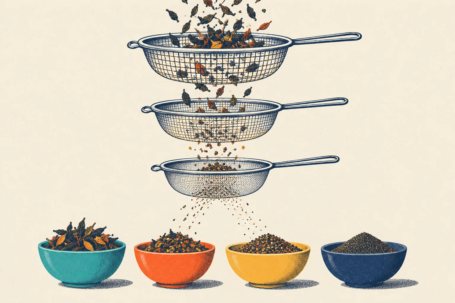
Look at the picture. Loose tea pours in at the top. Each sieve holds some pieces back and lets the rest through. At the bottom, the tea lands in four bowls, sorted by size. A SQL query works in the same way. Rows pour in from a table. Tests hold some of them back. What passes is sorted into groups, and each group is measured. By the end of this chapter, you will know which part of a query is the sieve and which part is the bowls. You will also know why Mia’s revenue came out almost twice too big.

Tables, rows and questions

A database keeps data in tables. A table is a grid, like a spreadsheet. Each row is one record, and each column is one fact about that record. In the orders table, one row is one order. Its columns include order_id, city, status and net_amount, the money the customer paid.

Chapter 1 called this the grain of a table: what one row stands for. Keep that word in mind. It is the most important word in this chapter.

A query is a question that you send to a database, written in SQL. The database answers with a new, small table, called the result.

To keep the examples small, the orders table in this chapter holds only the two weeks of the case, 31 August to 13 September: 91,818 orders of every status. These are the same rows that you can query yourself in “Try it”, below. Every result in this chapter is the real output of the query above it, run in DuckDB: a small database built for analysis, which can run inside a program or a web browser. The results use each order’s final status (see Chapter 1), so a few differ slightly from what Mia’s screen showed that Wednesday.

Here is the smallest useful query:

SELECT order_id, pickup_code, city, status, net_amount
FROM orders
LIMIT 3;

order_id	pickup_code	city	status	net_amount
4066824	E1001	harbor	completed	8.24
4066825	C1001	oldtown	completed	13.99
4066826	A1001	harbor	completed	8.74

Read it as English: select these five columns from the orders table, and stop after three rows. SELECT names the columns. FROM names the table. LIMIT 3 asks for three rows only. Theo likes LIMIT on a live database: it stops a careless query from pouring all 91,818 rows onto your screen. But LIMIT limits only the rows you get back, not the work. With ORDER BY or GROUP BY (you will meet both in a moment), the database must still read every row before it can return the first three. (Chapter 9 shows what that can cost.)

One warning. A table has no built-in order, so LIMIT 3 may return any three rows. Here, they happen to be the first three orders of the two weeks.

WHERE: the sieve

WHERE keeps only the rows that pass a test. Here, Mia asks for completed orders worth more than $1,000:

SELECT order_id, city, items_count, net_amount
FROM orders
WHERE status = 'completed'
  AND net_amount > 1000;

order_id	city	items_count	net_amount
4067207	riverside	193	1,161.25
4073506	harbor	190	1,082.50
4086755	harbor	400	2,013.75
4088630	riverside	400	2,264.50
4120309	harbor	400	2,466.70

Only 5 of the 91,818 rows passed the sieve. All 5 are bulk orders from corporate accounts, with 190 drinks or more. (Chapter 2 met these giant orders.)

AND joins two tests: a row passes only if both are true. OR lets a row pass if at least one test is true. Text values go in single quotes, like 'completed'. Numbers do not.

ORDER BY: put the answer in order

ORDER BY sorts the result by one or more columns. DESC means largest first. Without DESC, the sort runs from smallest to largest. Together with LIMIT, it gives you the top rows:

SELECT order_id, city, items_count, net_amount
FROM orders
WHERE status = 'completed'
ORDER BY net_amount DESC
LIMIT 3;

order_id	city	items_count	net_amount
4120309	harbor	400	2,466.70
4088630	riverside	400	2,264.50
4086755	harbor	400	2,013.75

Now LIMIT 3 means something: the three largest completed orders of the two weeks.

Aggregates: from many rows to one number

Now Mia’s real question: how many completed orders did Steep have last week? An aggregate is a function that turns many rows into one value. count(*) counts rows. sum(column) adds up a column. avg, min and max do what their names say.

SELECT count(*) AS orders
FROM orders
WHERE status = 'completed'
  AND order_date BETWEEN DATE '2026-09-07' AND DATE '2026-09-13';

orders
43,153

For the week before, she changed the two dates. On her screen that Wednesday, the two weeks had 45,622 and 43,406 completed orders: a change of −4.9%. Mia ticked the number in her notebook. For the first time, she did not have to take anyone’s word for it. (With final statuses, as in the result above, the weeks have 45,441 and 43,153 orders and the change is −5.0%; see Chapter 1.)

order_date is the local day in Steep’s cities: the date printed on the receipt. Its type is DATE: a day, with no time. BETWEEN includes both ends, so on a DATE column these dates cover seven full days.

On a column with a time, the same words are a trap. created_at_local is a timestamp, a date and a time. created_at_local BETWEEN '2026-09-07' AND '2026-09-13' stops at midnight at the start of 13 September, so all of Sunday is lost: the count is 37,165, not 43,153. For timestamps, write a closed start and an open end: created_at_local >= DATE '2026-09-07' AND created_at_local < DATE '2026-09-14'.

GROUP BY: the bowls

One number is useful. One number for each kind of row is often more useful. GROUP BY sorts the rows that passed WHERE into groups, like the tea in the bowls. Then each aggregate runs once per group, and the result has one row per group.

SELECT status, count(*) AS orders
FROM orders
WHERE order_date BETWEEN DATE '2026-09-07' AND DATE '2026-09-13'
GROUP BY status
ORDER BY orders DESC;

status	orders
completed	43,153
cancelled	1,149
refunded	470

Last week, customers placed 44,772 orders. Of these, 1,149 were cancelled, and 470 were refunded after they were completed.

One rule comes with GROUP BY. Every column in SELECT must either be in GROUP BY or sit inside an aggregate. Otherwise, the database does not know which of the many values in a bowl to show you.

Written in one order, run in another

You write SELECT first, but the database cannot start there. It must first know which table to read. So the database works through a query in a different order from the way you write it:

FROM: take the table. (The tea pours in.)
WHERE: keep the rows that pass. (The sieves.)
GROUP BY: sort the rows into groups, and compute the aggregates for each group. (The bowls, each one weighed.)
SELECT: choose and name the columns of the result.
ORDER BY: sort the result.
LIMIT: cut it short.

This order explains many error messages. For example, WHERE cannot use count(*), because WHERE runs before the groups exist. To filter whole groups after counting, SQL has a separate clause, HAVING, which runs after GROUP BY. And a name that you give a column in SELECT, with AS, is not known yet in WHERE, because SELECT comes later.

JOIN: putting two tables together

The orders table has the money, but not the drinks. The drinks are in order_items, and its grain is different. One row of order_items is one order line: one kind of drink in an order, with a quantity, qty. Two milk teas and one matcha make one order with two lines. The milk-tea line has a qty of 2.

Every line carries the order_id of its order. That shared column is how the two tables find each other. A join puts two tables side by side and pairs their rows on a condition that you write after ON:

SELECT o.order_id, o.net_amount, i.line_no, i.qty, i.unit_price
FROM orders AS o
JOIN order_items AS i ON i.order_id = o.order_id
WHERE o.order_id = 4066840;

order_id	net_amount	line_no	qty	unit_price
4066840	18.79	1	1	4.50
4066840	18.79	2	1	5.50
4066840	18.79	3	1	5.25

Order 4066840 had 3 lines, so the join returned 3 rows. Look at the net_amount column. The order’s money, $18.79, appears on every line. It belongs to the order, not to the line, so the join copied it onto each line.

AS o and AS i give the two tables short nicknames, called aliases. o.net_amount means “the net_amount column of orders”.

Two kinds of join cover most daily work:

An inner join (JOIN, or INNER JOIN) keeps only the rows that found a partner in the other table.
A left join (LEFT JOIN) keeps every row of the first table, the left one, even when it found no partner. Where there is no partner, the columns from the other table are empty.

The left join comes back later in this chapter. First, the trap.

The fan-out trap

Here is the query Mia ran on Wednesday morning:

SELECT count(*) AS orders,
       sum(o.net_amount) AS revenue,
       sum(i.qty) AS drinks
FROM orders AS o
JOIN order_items AS i ON i.order_id = o.order_id
WHERE o.status = 'completed'
  AND o.order_date BETWEEN DATE '2026-08-31' AND DATE '2026-09-06';

orders	revenue	drinks
65,923	1,034,175.15	77,393

Three numbers came back. Only one of them was right.

drinks (77,393) is right. Drinks live on the order lines, and the query added up order lines.
orders (65,923) is wrong. count(*) counted the rows after the join. Those rows are lines, not orders.
revenue ($1,034,175.15) is wrong. Each order’s money was copied onto each of its lines, and then added up once per line. An order with three lines was counted three times.

This is the fan-out: a join that turns one row into many, the way a folded paper fan opens into many folds. It happens whenever one row on one side matches several rows on the other side. In the week before, 36% of the completed orders had more than one line. So 45,441 orders became 65,923 rows: about 1.45 rows per order. The revenue grew even more, by 1.84 times. Big orders have many lines, so the biggest amounts were copied the most times. Bulk orders from corporate accounts had 5.5 lines on average; ordinary orders had 1.4.

The query had no error. Every number in the result is correct for the question it answers. The question was asked at the wrong grain. Mia wanted facts about orders, but the joined table has one row per order line.

There is a quick test for a fan-out. Count the rows, and count the different order IDs. count(DISTINCT o.order_id) counts each different value once:

SELECT count(*) AS joined_rows,
       count(DISTINCT o.order_id) AS orders
FROM orders AS o
JOIN order_items AS i ON i.order_id = o.order_id
WHERE o.status = 'completed'
  AND o.order_date BETWEEN DATE '2026-08-31' AND DATE '2026-09-06';

joined_rows	orders
65,923	45,441

If the two numbers differ, the join copied rows.

Two ways out

The first way is to ask each question at its own grain. Count the orders and add up the money in orders, with no join. Add up the drinks from order_items joined to orders (you need the status and the date). Each line has exactly one order, so this join copies nothing. Two small queries give two right answers.

The second way keeps one query. First, shrink order_items to one row per order. Then join. A CTE (a common table expression) lets you write this in readable steps. It starts with WITH, gives a small query a name, and lets the main query use that name as if it were a table:

WITH drinks_per_order AS (
  SELECT order_id, sum(qty) AS drinks
  FROM order_items
  GROUP BY order_id
)
SELECT count(*) AS orders,
       sum(o.net_amount) AS revenue,
       sum(d.drinks) AS drinks
FROM orders AS o
JOIN drinks_per_order AS d ON d.order_id = o.order_id
WHERE o.status = 'completed'
  AND o.order_date BETWEEN DATE '2026-08-31' AND DATE '2026-09-06';

orders	revenue	drinks
45,441	563,366.59	77,393

Now one row per order meets one row per order, and nothing fans out: 45,441 orders, $563,366.59 of revenue, and the same 77,393 drinks. Mia wrote a rule at the top of a clean page: Before a join, write down the grain of each side. After a join, check that the count did not grow.

When a partner is missing: LEFT JOIN and NULL

Theo came back at lunch and read over her shoulder. “Good. Now ask a question where some rows have no partner.”

He picked one store and one quiet hour: store RVS-02 on Sunday 13 September, before 8:00 in the morning, when 3 orders came in. Which of the 12 drinks on the menu did those customers order? The CTE early collects the order lines of that hour. Then the main query joins the full menu to it with a left join, so that every drink stays in the result:

WITH early AS (
  SELECT i.menu_item_id, i.qty
  FROM orders AS o
  JOIN order_items AS i ON i.order_id = o.order_id
  WHERE o.store_id = 'RVS-02'
    AND o.order_date = DATE '2026-09-13'
    AND hour(o.created_at_local) < 8
)
SELECT m.name, sum(e.qty) AS drinks
FROM menu_items AS m
LEFT JOIN early AS e ON e.menu_item_id = m.menu_item_id
GROUP BY m.menu_item_id, m.name
ORDER BY drinks DESC NULLS LAST, m.name;

name	drinks
Brown Sugar Boba Milk	1
Classic Milk Tea	1
Jasmine Green Tea	1
Oolong Milk Tea	1
Passion Fruit Green Tea	1
Taro Milk Tea	1
Cheese Foam Black Tea	NULL
Lychee Oolong	NULL
Mango Fruit Tea	NULL
Matcha Latte	NULL
Strawberry Matcha Cloud	NULL
Thai Tea	NULL

6 drinks were ordered. The other 6 have an empty drinks cell, shown as NULL. An inner join would have dropped those 6 rows without a word. The left join keeps them, so you can see what is missing.

NULL is SQL’s mark for “no value here”. It is not zero, and it is not empty text. It means missing or unknown. NULL has three habits that surprise most people once:

Aggregates skip it. sum(e.qty) and count(e.qty) ignore NULL cells, but count(*) still counts the row. If nothing is left to add, sum gives NULL, not 0 (count gives 0). That is where the NULLs in the result above come from. To show 0 instead, write coalesce(sum(e.qty), 0) AS drinks.
Nothing equals NULL, not even another NULL. The test e.qty = NULL is never true. Write e.qty IS NULL instead.
A calculation with NULL gives NULL: NULL + 1 is NULL. To turn NULL into a number, write coalesce(e.qty, 0). It returns the first value that is not NULL.

Add WHERE e.menu_item_id IS NULL to the left join, and the result keeps only the drinks that nobody ordered. A left join that keeps only the rows with no partner has its own name: an anti-join. In Chapter 7, Mia uses one to find orders that have no order_completed event in the warehouse.

Window functions: looking at the neighbours

GROUP BY squeezes each group into one row. Sometimes you want to keep every row and still look at the other rows in its group. A window function does this. It computes a value for each row from a “window” of related rows, and every row stays in the result.

You write a window function with OVER (...). Inside, PARTITION BY says which rows belong together, and ORDER BY says in which order to look at them.

Numbering rows. row_number() gives the rows in each partition the numbers 1, 2, 3 and so on. Here, Mia asks for the largest order, by money, in each city:

WITH ranked AS (
  SELECT city, order_id, items_count, net_amount,
         row_number() OVER (
           PARTITION BY city
           ORDER BY net_amount DESC, order_id
         ) AS rn
  FROM orders
  WHERE status = 'completed'
)
SELECT city, order_id, items_count, net_amount
FROM ranked
WHERE rn = 1
ORDER BY city;

city	order_id	items_count	net_amount
harbor	4120309	400	2,466.70
northgate	4067215	180	955.25
oldtown	4125873	128	778.35
riverside	4088630	400	2,264.50

All four are bulk orders from corporate accounts again. The query needs two steps. A window function is computed in the SELECT step, and WHERE runs before that step. So the first step numbers the rows, and the second step keeps the rows numbered 1.

The second sort column, order_id, is a tie-breaker. If two orders in a city had the same amount, row_number() would otherwise pick one of them in no fixed way, and the answer could change from one run to the next.

The same pattern answers many everyday questions. For each customer’s first order, partition by user_id and order by created_at_local, then order_id. For the three newest orders in each store, partition by store_id, order by time with DESC, and keep rn <= 3.

Running totals. sum(...) OVER (...) adds up the rows so far, in order. Mia used it to let the two weeks race each other, day by day. The query also uses CASE WHEN ... THEN ... ELSE ... END, SQL’s “if, then, otherwise”: here it labels each day 'before' or 'last'.

WITH daily AS (
  SELECT order_date,
         CASE WHEN order_date <= DATE '2026-09-06'
              THEN 'before' ELSE 'last' END AS week,
         count(*) AS orders
  FROM orders
  WHERE status = 'completed'
  GROUP BY order_date, week
)
SELECT week, order_date, orders,
       sum(orders) OVER (
         PARTITION BY week
         ORDER BY order_date
       ) AS running_total
FROM daily
ORDER BY order_date;

week	order_date	orders	running_total
before	2026-08-31	5,458	5,458
before	2026-09-01	6,124	11,582
before	2026-09-02	6,188	17,770
before	2026-09-03	6,744	24,514
before	2026-09-04	7,546	32,060
before	2026-09-05	7,306	39,366
before	2026-09-06	6,075	45,441
last	2026-09-07	5,265	5,265
last	2026-09-08	5,879	11,144
last	2026-09-09	6,045	17,189
last	2026-09-10	6,188	23,377
last	2026-09-11	6,849	30,226
last	2026-09-12	6,939	37,165
last	2026-09-13	5,988	43,153

By Wednesday, the week before had reached 17,770 completed orders, and last week only 17,189. Last week was behind from its first day, and it fell further behind on every day after that. The drop was not one bad day. It was spread over the whole week.

Two details in this query. First, week is a name made in SELECT, yet GROUP BY uses it. DuckDB allows this; not every database does. Elsewhere, repeat the whole CASE expression in GROUP BY. Second, for a running total that is always safe, write ROWS BETWEEN UNBOUNDED PRECEDING AND CURRENT ROW after the ORDER BY. (The box below explains why.)

The question Mia came for

Now Mia could ask the question that had brought her to the database. The dashboard said orders fell 12.0%. Her own count said they fell about 5%. About 7 points of the drop lay between the two. That was Clue 1. But where did it live?

The dashboard counts order_completed events: a message that the app sends when a customer pays. Theo keeps a daily summary of the app’s messages, events_daily. It has one row per day, platform, app version and event name, and the number of events in the column events. (A few messages arrive twice; the summary counts each one once. Chapter 8 shows how.) Added up, its order_completed events give exactly the dashboard’s numbers: 46,924 in the week before and 41,289 last week.

A platform is the kind of app that a customer uses: the iPhone app (iOS), the Android app, or the website. Mia counted both sources by platform and put them side by side, with two CTEs and a join:

WITH db AS (
  SELECT platform,
         count(*) FILTER (WHERE order_date <= DATE '2026-09-06') AS w1,
         count(*) FILTER (WHERE order_date >= DATE '2026-09-07') AS w2
  FROM orders
  WHERE status = 'completed'
    AND order_date BETWEEN DATE '2026-08-31' AND DATE '2026-09-13'
  GROUP BY platform
),
dash AS (
  SELECT platform,
         sum(events) FILTER (WHERE event_date <= DATE '2026-09-06') AS w1,
         sum(events) FILTER (WHERE event_date >= DATE '2026-09-07') AS w2
  FROM events_daily
  WHERE event_name = 'order_completed'
    AND event_date BETWEEN DATE '2026-08-31' AND DATE '2026-09-13'
  GROUP BY platform
)
SELECT platform,
       round(100.0 * (db.w2 - db.w1) / db.w1, 1) AS database_pct,
       round(100.0 * (dash.w2 - dash.w1) / dash.w1, 1) AS dashboard_pct
FROM db
JOIN dash USING (platform)
ORDER BY platform;

platform	database_pct	dashboard_pct
android	-4.9	-4.5
ios	-5.3	-17.4
web	-3.7	-4.2

Two small new things are in this query. FILTER (WHERE ...) makes an aggregate count only some of the rows in each group, so one row can hold both weeks. (Not every database has FILTER. The longer form count(CASE WHEN ... THEN 1 END) works everywhere.) And 100.0 instead of 100 keeps the division in decimals: in some databases, 7 / 2 is 3.

On Android and the web, the two sources agree to within about half a percentage point. On iOS, they do not. The database says iOS orders fell 5.3%, much like the other platforms. The dashboard says they fell 17.4%.

To see how much of the gap each platform holds, Mia measured each platform’s change on the dashboard and in the database, both as a share of that source’s whole week before, and took the difference. The pieces add up exactly to the gap. Of the 7.0-point gap, iOS alone explains about 7.1. Android and the web make it about 0.1 smaller. So the gap between the dashboard and the database is almost all iOS. (The box below shows the formula.)

Mia took her phone out of her bag and looked at it for a moment. It was an iPhone. Then she wrote in her notebook: Clue 1 lives on iOS. Suspect: something that stops iPhone orders from reaching the dashboard. Not known yet: what, or since when.

Under the hood

The full order of a query. The database works through the clauses in this order: FROM and JOIN → WHERE → GROUP BY → HAVING → SELECT (window functions are computed here) → DISTINCT → ORDER BY → LIMIT. Real databases may run the steps in a smarter order inside, but the result must be the same as if they followed this one.

How many rows a join returns. Take one value $k$ of the join key. If it appears $a_k$ times on the left and $b_k$ times on the right, an inner join returns $a_k \times b_k$ rows for it, and a left join returns $a_k \times \max(b_k, 1)$. Over all keys,

\[\text{rows of an inner join} = \sum_k a_k\, b_k .\]

In a left join, a sum over a left-table column is sure to stay the same when every $b_k \le 1$. In an inner join, every $b_k$ must be exactly 1.

Why revenue grew more than the rows. After the fan-out, order $j$ with $L_j$ lines and amount $x_j$ is counted $L_j$ times. So

\[\frac{\text{fanned-out revenue}}{\text{true revenue}} = \frac{\sum_j L_j x_j}{\sum_j x_j},\]

an average of $L_j$ weighted by money. The row factor $\sum_j L_j / J$, where $J$ is the number of orders, is a plain average. When big orders have more lines, the weighted average is larger: here 1.84 against 1.45.

Running totals and ties. When OVER has an ORDER BY and no frame, the default frame is RANGE BETWEEN UNBOUNDED PRECEDING AND CURRENT ROW. “Range” means the sum includes every row tied with the current one on the ORDER BY value, so two rows with the same order_date get the same running total, which already includes both. ROWS BETWEEN UNBOUNDED PRECEDING AND CURRENT ROW counts rows one by one instead. Without any ORDER BY in OVER, the frame is the whole partition, so every row gets the partition’s total.

Ranking with ties. row_number() gives every row its own number; among tied rows, the order is not fixed unless you add a tie-breaker. rank() gives tied rows the same number and then skips (1, 1, 3). dense_rank() does not skip (1, 1, 2). So with rank() or dense_rank(), a filter such as rn <= 3 can return more than three rows per group. Some databases, such as DuckDB and Snowflake, offer QUALIFY, which filters on a window function without a second step.

NULL logic. A comparison with NULL is neither true nor false, but unknown. WHERE keeps a row only when its test is true, so rows whose test is unknown are dropped too. That is why city <> 'harbor' does not return rows where city is NULL.

Points by platform. Write $D_p^{1}, D_p^{2}$ for the dashboard’s count on platform $p$ in the two weeks, and $B_p^{1}, B_p^{2}$ for the database’s. Each platform’s share of each source’s week-over-week change is

\[c_p = \frac{D_p^{2} - D_p^{1}}{\sum_q D_q^{1}} - \frac{B_p^{2} - B_p^{1}}{\sum_q B_q^{1}},\]

and the $c_p$ add up exactly to the dashboard change minus the database change. In points, iOS gives −7.1, Android 0.1, and the web −0.1: together −7.0.

Try it

Steep’s two weeks, in your browser. Four tables are loaded: orders (every order from 31 August to 13 September), order_items (their lines), menu_items (the twelve drinks) and events_daily (the app’s daily message counts). Pick a starting query, change it if you like, and press “Run query”.

Show the code

sqlDb = DuckDBClient.of({
  orders: FileAttachment("../data/out/web/orders_w1w2.parquet"),
  order_items: FileAttachment("../data/out/web/order_items_w1w2.parquet"),
  menu_items: FileAttachment("../data/out/web/menu_items.parquet"),
  events_daily: FileAttachment("../data/out/web/events_daily.parquet")
})

Show the code

viewof sqlText = {
  const input = Inputs.textarea({value: sqlPreset, rows: 12, width: "100%", monospace: true, submit: "Run query"});
  const box = input.querySelector("textarea");
  box.style.fontSize = "0.78rem";
  box.style.lineHeight = "1.4";
  return input;
}

Show the code

sqlResult = {
  try {
    const rows = await sqlDb.query(sqlText);
    const schema = rows.schema || [];
    return {rows: Array.from(rows, r => (typeof r.toJSON === "function" ? r.toJSON() : r)), schema, error: null};
  } catch (e) {
    return {rows: [], schema: [], error: String(e && e.message ? e.message : e)};
  }
}

Show the code

// Turn the browser database's values into plain text, the way the chapter's tables show them.
sqlFormat = {
  const SHOW_MAX = 500;
  // DECIMAL columns arrive as 128-bit integers plus a scale, e.g. "Decimal[38e+2]".
  const scaleOf = t => { const m = /Decimal\[\d+e([+-]?\d+)\]/.exec(t || ""); return m ? Number(m[1]) : null; };
  const decimal = (v, scale) => {
    if (typeof v === "number") return v;
    if (typeof v === "bigint") return Number(v) / 10 ** scale;
    if (ArrayBuffer.isView(v)) {
      let big = 0n;
      for (let i = v.length - 1; i >= 0; i--) big = (big << 32n) | BigInt(v[i]);
      if (v[v.length - 1] & 0x80000000) big -= 1n << BigInt(32 * v.length);
      return Number(big) / 10 ** scale;
    }
    return Number(v);
  };
  const pad = x => String(x).padStart(2, "0");
  const when = d => {
    const day = `${d.getUTCFullYear()}-${pad(d.getUTCMonth() + 1)}-${pad(d.getUTCDate())}`;
    const time = `${pad(d.getUTCHours())}:${pad(d.getUTCMinutes())}:${pad(d.getUTCSeconds())}`;
    return time === "00:00:00" ? day : `${day} ${time}`;
  };
  const text = (v, field) => {
    if (v == null) return "NULL";
    const scale = scaleOf(field && field.databaseType);
    if (scale !== null) {  // money and other exact decimals keep their decimal places
      const x = decimal(v, scale);
      return x.toLocaleString("en-US", {minimumFractionDigits: scale, maximumFractionDigits: scale});
    }
    if (field && field.type === "date" && !(v instanceof Date)) v = new Date(Number(v));
    if (v instanceof Date) return when(v);
    if (typeof v === "bigint") v = Number(v);
    if (typeof v === "number") {
      if (Number.isInteger(v)) return /_id$/.test(field ? field.name : "") ? String(v) : v.toLocaleString("en-US");
      return v.toLocaleString("en-US", {maximumFractionDigits: 2});
    }
    if (typeof v === "boolean") return String(v);
    return String(v);
  };
  return {SHOW_MAX, text};
}

Show the code

{
  if (sqlResult.error) {
    return htl.html`<p style="color:#b8401c;font-family:Inter,system-ui,sans-serif;font-size:0.85rem">The query did not run: ${sqlResult.error}</p>`;
  }
  const {rows, schema} = sqlResult;
  const fields = new Map(schema.map(f => [f.name, f]));
  const columns = rows.length ? Object.keys(rows[0]) : schema.map(f => f.name);
  const names = schema.map(f => f.name);
  const repeated = [...new Set(names.filter((name, i) => names.indexOf(name) !== i))];
  const warning = repeated.length
    ? htl.html`<p style="color:#b8401c;font-size:0.82rem;margin:0.2rem 0">Some columns share a name
        (${repeated.join(", ")}), so only the last column of each name is shown. Give each column its own
        name with AS.</p>`
    : "";
  const shown = rows.slice(0, sqlFormat.SHOW_MAX).map(r =>
    Object.fromEntries(columns.map(c => [c, sqlFormat.text(r[c], fields.get(c))])));
  const note = rows.length > sqlFormat.SHOW_MAX
    ? `${rows.length.toLocaleString("en-US")} rows; showing the first ${sqlFormat.SHOW_MAX}.`
    : `${rows.length.toLocaleString("en-US")} row${rows.length === 1 ? "" : "s"}.`;
  const right = Object.fromEntries(columns.map(c => {
    const t = fields.get(c) && fields.get(c).type;
    return [c, t === "integer" || t === "number" ? "right" : "left"];
  }));
  return htl.html`<div>
    <p style="font-size:0.82rem;margin:0.2rem 0">${note}</p>
    ${warning}
    ${Inputs.table(shown, {rows: 14, layout: "auto", align: right})}
  </div>`;
}

Things to try:

Run “Mia’s first revenue query”, then “The fix: a CTE”. Compare the three numbers.
In “The gap by platform”, replace everything from the last SELECT to the end with the lines below. They show the raw counts behind the percentages. (Both CTEs have columns called w1 and w2, so each one needs a new name with AS.)
```
SELECT platform,
       db.w1 AS db_w1, db.w2 AS db_w2,
       dash.w1 AS dash_w1, dash.w2 AS dash_w2
FROM db JOIN dash USING (platform);
```
In “LEFT JOIN: drinks nobody ordered”, change LEFT JOIN to JOIN. Which rows disappear?
In “A1024: a label, not a key”, count how many different orders share one receipt code.

Common traps

Joining two grains. A join between one row per order and one row per line copies every order value. Write down the grain of each side before you join. After the join, compare count(*) with count(DISTINCT key).
Fixing a fan-out with sum(DISTINCT ...). It removes copies of the same amount, not of the same order. Two different orders of $8.24 would be counted once. Aggregate to the right grain instead.
= NULL. It is never true. Use IS NULL or IS NOT NULL.
A left join that quietly becomes an inner join. A test on the right table in WHERE that is never true for NULL, such as WHERE e.qty > 0, drops the rows where e.qty is NULL. Put such tests in the ON condition, or in the CTE, instead.
LIMIT without ORDER BY. You get some rows, not the first or the best ones.
A label is not a key. In these two weeks alone, pickup_code = 'A1024' matches 56 different orders. Join and filter on order_id, the real key.
BETWEEN on a timestamp. It stops at midnight at the start of the last day. Use >= the first day and < the day after the last.
Whole numbers that divide badly. In some databases, 7 / 2 is 3. Write 100.0 * a / b for percentages.

Audit Instinct · CAATs are SQL in disguise

Many auditors already write queries without calling them that. Computer-assisted audit techniques (CAATs) are tools, such as ACL and IDEA, that test a whole data file instead of a sample. Their main commands map onto SQL. An extraction is WHERE. A summarization is GROUP BY with count and sum. Joining two files is a JOIN.

A join is a three-way match. In the purchasing cycle, an auditor matches the purchase order, the goods received note and the supplier’s invoice. Matching them on the purchase order number is a join across three tables. A purchase order with no receipt is the row that a left join keeps and an inner join hides.

A fan-out is the classic double count. One purchase order often has several deliveries. Join purchase orders to receipts, add up the purchase order amount, and an order with three deliveries is counted three times. The auditor’s fix is Mia’s fix: bring both sides to the same grain first. Total the receipts per purchase order, then match.

Interview Corner

Q1. Find the three largest orders in each city.

A short answer

Number the rows inside each city with a window function, then keep the first three:

WITH ranked AS (
  SELECT city, order_id, net_amount,
         row_number() OVER (
           PARTITION BY city
           ORDER BY net_amount DESC, order_id
         ) AS rn
  FROM orders
)
SELECT * FROM ranked WHERE rn <= 3;

Add a tie-breaker, such as ORDER BY net_amount DESC, order_id, so the answer is the same on every run. Then ask what should happen with ties: rank() and dense_rank() keep tied rows together, and then <= 3 can return more than three rows (see Under the hood).

Q2. Table A has 1,000 rows. You LEFT JOIN table B. How many rows can come back?

A short answer

At least 1,000: a left join keeps every row of A. Exactly 1,000 if each row of A matches at most one row of B. More than 1,000 if some rows of A match several rows of B: that is a fan-out. An inner join can return anything from 0 rows (no matches) up to 1,000 times the number of rows in B. Then mention the trap. A WHERE test on B that can never be true for NULL, such as =, > or IN, turns the left join into an inner join. IS NULL instead keeps only the rows with no partner: the anti-join.

Q3. Why does my SUM double after a join?

A short answer

Because the join changed the grain. If one order matches three lines, the order’s amount appears three times, and SUM adds all three. Check it by comparing count(*) with count(DISTINCT order_id). Fix it by adding up the amount at its own grain, without the join, or by aggregating the “many” side to one row per key before the join (a CTE helps). Do not fix it with SUM(DISTINCT amount): two different orders with the same amount would be merged.

Reported change: −12.0% orders, the week of 7 September compared with the week before (CEO dashboard).

Explained so far: 0 of the 12 points.

Suspects: measurement on iOS (not proved). Mia’s own SQL confirms finance’s count: completed orders changed by −5.0% (final statuses, see Chapter 1). About 7.0 points lie between the database and the dashboard, and iOS holds about 7.1 of them: on iOS, the database says −5.3% and the dashboard −17.4%.

Ruled out: smaller baskets (Chapter 2). Android and the web as the home of the gap (this chapter).

Open questions: What on iOS stops orders from reaching the dashboard, and since when? (Chapter 5 dates it; Chapter 6 follows iPhone customers through the app.) Is the database’s fall of about 5% a fair comparison? (Part III.)

New evidence: receipt A1024, ordered on Mia’s iPhone; the platform table above.

Recap

A query is a precise question. SELECT says what, FROM says where, WHERE says which rows, GROUP BY sorts them into groups, and aggregates measure each group.
Every table has a grain. A join between two grains copies rows: a fan-out. Bring both sides to the same grain before you join, and check the row count after.
A left join keeps rows that have no partner and marks the gaps with NULL. A window function looks at the neighbouring rows without squeezing them into one.

English	中文
query	查询
table / row / column	表 / 行 / 列
grain	粒度
aggregate	聚合
GROUP BY	分组
join	连接
inner join / left join	内连接 / 左连接
alias	别名
fan-out (join)	扇出 / 重复计数
CTE (common table expression)	公用表表达式
NULL	空值
anti-join	反连接
window function	窗口函数
running total	累计值
CAATs	计算机辅助审计技术

Tables, rows and questions

WHERE: the sieve

ORDER BY: put the answer in order

Aggregates: from many rows to one number

GROUP BY: the bowls

Written in one order, run in another

JOIN: putting two tables together

The fan-out trap

Two ways out

When a partner is missing: LEFT JOIN and NULL

Window functions: looking at the neighbours

The question Mia came for

Try it

Common traps

Recap

Further reading