On Monday afternoon, Mia did what auditors do with a number they have not checked yet. She asked for it again, from someone else.
She sent one short message to three teams: “How many orders did Steep have last week, from Monday 7 to Sunday 13 September?”
The first answer was already on the wall in Dana’s office. The CEO’s dashboard said 41,289.
Finance replied twenty minutes later, with a spreadsheet: 43,494.
Operations, the team that runs the stores and the couriers, replied last. They sent a photo of the whiteboard in their office: 44,772.
Mia wrote the three numbers in her notebook, one under the other. They were close, but they were not the same. The largest was 3,483 orders above the smallest. That is more than half of an ordinary day at Steep.
Theo stopped at her desk with a mug of tea. He read the page upside down.
“Three teams, three numbers,” he said. “Welcome to data.”
“Which one is right?”
“Maybe all of them.” He took a paper napkin from his pocket and drew a cup. Then he drew three lamps around it, and three shadows on a wall behind it: a circle, a rectangle and a trapezoid. “One cup. Light it from three sides and you get three shadows. Each shadow is real. None of them is the cup.”
“So each team sees the orders from a different side.”
“Each team has a rule for what counts as an order. Ask for the rule, not for the number.” He finished his tea. “And ask before you compare. People who compare first end up in long meetings.”
Mia turned to a new page and wrote one line at the top: Compare the rules before you compare the numbers.
ImportantThe big idea
A metric is a definition, not a fact. Before you compare two numbers, compare their definitions.
Look at the picture above. One cup stands on a table. Three lamps shine on it: a teal lamp from the left, a mustard lamp from the right, and a tomato lamp from below. On the wall, the cup throws three shadows of three different shapes. The cup never changes. Only the light changes. In this chapter, the cup is last week’s orders, and each lamp is one team’s way of counting them.
Measurements and metrics
Start with the smallest piece. When Mia paid for her tea this morning, Steep’s orders database saved one row: order number 4158971, store HBR-01, placed at 08:47:21, one drink. A row like this is a measurement: one recorded fact about one thing that happened.
Nobody runs a company by reading single rows. Dana wants one number for the whole week. A metric is a number that sums up many measurements with a fixed rule. “Orders last week” is a metric. “Revenue per day” is another.
The rule is the metric’s definition. Chinese data teams call it 口径 (kǒujìng). The word first meant the width of an opening, such as the mouth of a bottle. In data work, it means the rule that decides what goes into a number.
A measurement can be wrong. A clock can run slow, and an app can fail to send a message. A metric can be wrong in the same ways, and in one more way: its rule can be different from the rule you think it has. Two metrics with the same name and different rules are two different metrics. They only share a name.
Five questions for any definition
Mia did not ask the three teams whether their numbers were right. She asked them how they counted. Then she sorted their answers under five questions. You can ask the same five questions about any metric.
1. What counts?
A Steep order can end in three ways. The database keeps a status for every order: a field that says how the order ended.
completed: the drink was made and paid for, and Steep kept the money.
cancelled: the customer paid, then cancelled a few minutes later, before the drink was made. The money went back.
refunded: the order was completed, but later Steep gave the money back.
Finance counts only completed orders, because finance counts money that Steep kept. Operations counts all three, because every order printed a ticket in a store and took a worker’s time, even the orders that were cancelled later. A third choice sits in between: count every order that was made, even if it was refunded later. This book calls these fulfilled orders.
2. Where is it counted?
At Steep, an order is recorded in two places.
The first place is the orders database, the system that takes the money. Finance and operations both count rows there.
The second place is the app. When a customer does something in the app, the app sends a short message to Steep’s servers. Such a message is an event: a small record that says “this happened”, with who, what and when. When a payment goes through, the app sends an event called order_completed. The dashboard counts these events. Its order count comes only from them.
3. When?
Every count covers a stretch of time, and that needs three choices.
Which clock? A time zone is a region that uses the same clock time. Computers often store times in UTC (Coordinated Universal Time), the world’s reference clock. Steep’s four cities are 7 hours behind UTC. So at 5 pm in Harbor, the date in UTC has already changed to the next day.
Which day starts the week? All three teams at Steep use Monday to Sunday. Many calendars start the week on Sunday.
Which moment? An order has several times: when the customer tapped “Pay”, when Steep’s server received the event, and when the status last changed. The dashboard uses the moment the event happened, by the phone’s clock. Finance and operations use the moment the order was placed.
A definition also needs an as-of time: the moment you read the data. Finance’s spreadsheet came from the orders database as it stood at the start of that Monday. But refunds keep coming after a week ends. From June to October, 65% of refunds came within five days of the order. The rest came later, up to 40 days after it, for example when a customer disputed the payment with the bank. Each refund turns a completed order into a refunded one, so finance’s count for a week keeps shrinking for weeks.
NoteHow this book counts order status
This book follows one rule, and later chapters point back to it.
Headline numbers (case boards, charts and tables) use each order’s final status: the status it has at the end of the data, in late October.
In a scene, a character sees the numbers of that day. Mia cannot see refunds that have not happened yet.
So you will meet finance’s definition with three slightly different results for the same two weeks:
Read on
Last week’s completed orders
Change from the week before
Monday 14 September, start of the day (this chapter)
43,494
−4.7%
Wednesday 16 September, 9 am (Chapter 3)
43,406
−4.9%
End of the data: final statuses (every headline number)
43,153
−5.0%
The orders did not change. Only their statuses did: by the end of October, 341 of last week’s orders and 186 from the week before had been refunded after that Monday. Every reading says the same thing: a fall of about 5%. Chapter 11 shows how to rebuild the database as it stood at any past moment.
4. One row = one what?
Before you count rows, find out what one row stands for. This is the table’s grain. In the orders table, one row is one order. In the table of order lines, one row is one line on the receipt: one kind of drink, with a quantity. In the app’s events, one row is one event, and a few events arrive twice (Chapter 8 shows why). The dashboard removes these copies before it counts. Without that step, it would have counted 241 orders too many in these two weeks.
A related choice is the unit: what you add up. “How much did Steep sell?” has more than one honest answer. Finance counts orders. A store manager might add up drinks, because drinks are what the staff make. The grain stays the same, one row per order, but each row now adds its number of drinks. Last week’s completed orders held 71,310 drinks.
5. Who is included?
The population of a metric is the full set of things it covers. Does “orders” include the 236 corporate accounts that Steep had that Monday, the companies that order tea for a whole office? Other businesses also ask about staff orders and test orders made by the app team. At Steep, all three teams count every customer, so this question did not split them this time.
Three teams, side by side
Here are the three answers to the five questions.
Question
Dashboard
Finance
Operations
What counts?
Every order with an order_completed event in the warehouse
Orders with status completed
Every order, any status
Where?
App events
Orders database
Orders database
When?
Day the event happened, Steep time, Monday to Sunday
Day the order was placed, Steep time, Monday to Sunday
Same as finance
One row =
One event (copies removed)
One order
One order
Who?
Every customer
Every customer
Every customer
Look at the first row. The app sends order_completed at the moment of payment. At that moment, nobody knows yet whether the order will be cancelled or refunded. So the dashboard counts cancelled and refunded orders too, as operations does. In the week before, its count included 1,136 cancelled orders and 461 that were refunded later.
Then Mia asked each team for one more number: the same count for the week before, 31 August to 6 September. Now she could compare each team with itself. (The table uses final statuses, so finance’s numbers are a little lower than on its Monday spreadsheet. See “How this book counts order status” above.)
Team
The week before
Last week
Change
Dashboard (app events)
46,924
41,289
−12.0%
Finance (completed orders)
45,441
43,153
−5.0%
Operations (every order)
47,046
44,772
−4.8%
Every team saw a fall. But the dashboard’s fall was more than twice the size of the others.
Now look at the week before. Then, the dashboard was 1,483 orders above finance. Last week, it was 1,864 orders below. Two counts with different rules can sit a steady distance apart. When one moves from above the other to below it, that distance changed. Something changed in one of them: the orders it sees, or the way it counts.
Change one thing at a time
Mia did not try to explain all the gaps at once. She looked for two counts whose definitions differ in only one way.
The dashboard and operations are such a pair. Both count every order, whatever its status. Both use Steep’s days, Monday to Sunday. Both count every customer. The only difference is the where: the dashboard counts events from the app, and operations counts rows in the database.
Operations fell 4.8% and the dashboard 12.0%: 7.2 points apart, with the where as the only difference.
Every event on the dashboard belongs to exactly one order in the database, placed on the same day, and no order has two events. Mia checked this for all 88,213 events in the two weeks. So the dashboard counts the orders that have an event, and operations counts all orders. The difference is the orders without one: orders with no order_completed event in the warehouse.
Checking that two records of the same thing agree, and explaining every difference, is called reconciliation. Auditors do it every day. Here is Mia’s.
The week before
Last week
Operations: every order in the database
47,046
44,772
Dashboard: orders with an event
46,924
41,289
Orders with no event in the warehouse
122 (0.3%)
3,483 (7.8%)
In the week before, about 3 orders in a thousand had no event. Some loss like this is normal: phones lose their connection, apps crash, and messages get lost on the way. Last week, about 8 in a hundred had none. Where those events were lost, Mia could not tell yet. The data shows only that they are not in the warehouse.
This is how an auditor narrows down a problem. Hold everything still, change one thing, and watch the number. Here the one thing was the place where orders are counted, and the gap opened there.
Turning the other knobs
What about the other choices? Mia started from finance’s definition and changed one part at a time.
Show the code
rows = [ ("Operations: every status", operations, "db"), ("Weeks from Sunday to Saturday", sunday_weeks, "db"), ("UTC days instead of Steep days", utc_days, "db"), ("Fulfilled: refunds kept in", fulfilled, "db"), ("Finance: completed orders", finance, "db"), ("No corporate accounts", consumers, "db"), ("Drinks instead of orders", drinks, "unit"), ("Dashboard: app events", dashboard, "events"),]rows.sort(key=lambda r: -r[1].change)colors = {"db": bk.INK, "unit": bk.MUSTARD, "events": bk.TOMATO}fig, ax = bk.figure(8, 4.4)db_rows = [i for i, r inenumerate(rows) if r[2] =="db"]ax.axhspan(min(db_rows) -0.45, max(db_rows) +0.45, color=bk.GRID, alpha=0.45, lw=0)for i, (label, count, kind) inenumerate(rows): x =100* count.change ax.plot([x, 0], [i, i], color=colors[kind], lw=1, alpha=0.35) ax.scatter(x, i, s=70, color=colors[kind], zorder=3) ax.text(x -0.25, i, pct(count.change), ha="right", va="center", fontsize=9.5, color=bk.INK)ax.set_yticks(range(len(rows)), [r[0] for r in rows])ax.invert_yaxis()ax.axvline(0, color=bk.INK, lw=0.8)ax.set_xlim(100* dashboard.change -2.2, 0.6)ax.xaxis.set_major_formatter(lambda v, _: f"{v:.0f}%".replace("-", "−"))ax.grid(axis="y", visible=False)ax.grid(axis="x", visible=True)ax.set_xlabel("Change, last week compared with the week before")ax.set_title(f"Counted in the database, orders fell about {round(-100* finance.change)}%. "f"Counted from app events, {round(-100* dashboard.change)}%.")plt.show()
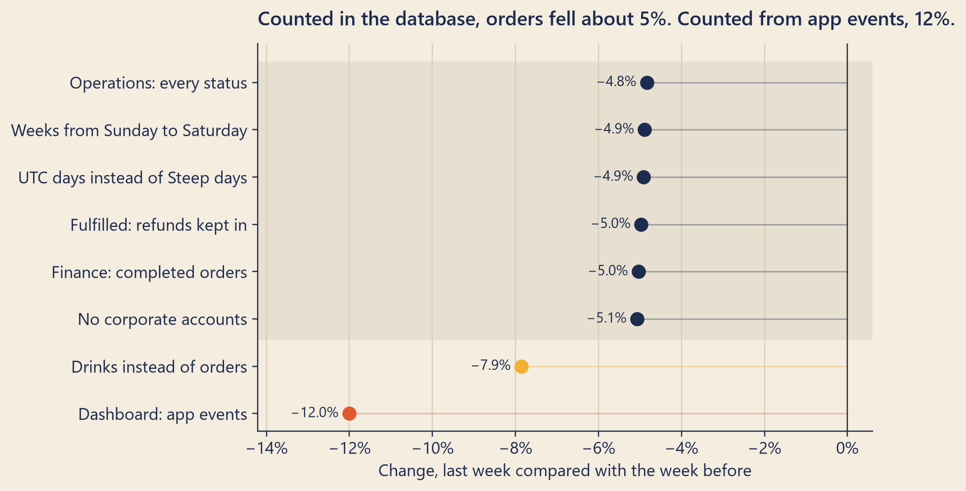
Figure 1: The change from the week before to last week, under eight definitions of the same metric. Each database row starts from finance’s definition and changes one part. The dashboard row is shown for comparison.
Every way of counting orders in the database tells the same story: a fall of about 5%, between −4.8% and −5.1%.
The choices still matter for the level of the count. Take the time zone. About 32% of Steep’s orders, about one in three, are placed after 5 pm, when the UTC date has already moved on. So a “day” in UTC holds a different set of orders from a day in Steep’s time. On Sunday 13 September, counting by UTC date gave 485 more completed orders than counting by Steep’s date.
Over a whole week, most of these moves cancel out, because the orders that leave one day enter the next one. Only the two ends of the week change. An order placed at 8 pm on Sunday 13 September belongs to last week by Steep’s clock. In UTC it is already Monday, so it moves into the next week. In the same way, Sunday-evening orders from 6 September move from the week before into last week.
The bigger danger comes when you combine tables. To join two tables is to match the rows of one with the rows of the other, for example by date. If you join a table kept in UTC with a table kept in local time, evening orders land on the wrong day, and nothing warns you.
The dashboard’s choice of moment barely matters here. Its events are dated by the phone’s clock, and the warehouse also records the day each event arrived. Only 25 of the 88,213 order_completed events in these two weeks arrived on a different day than they happened. (Chapter 14 is about events that arrive late.)
Drinks are different from orders. Drinks fell 7.9%, faster than orders. That is not a contradiction. Drinks and orders are different units, so they can move differently. Chapter 2 looks inside the orders to see why.
Only one definition says −12%, and it is the only one that counts app events.
A label is not a key
There was one more thing Mia wanted to check: her own receipt. She searched the orders table for pickup code A1024. She expected one row. She got 424, from the start of the data in June up to that Monday.
The Prologue explained that the letter on a pickup code stands for the store, and the number counts that store’s orders for the day. Each store’s counter starts again every morning. And in every city, the first store prints the letter A. So A1024 comes back every day, in every city. On Mia’s first day alone, four orders carried it, one in each of Steep’s four cities.
A key is a value that points to exactly one row in a table. In Steep’s orders table, the key is order_id, a number that the database gives each order and never uses again. A pickup code is a label: a name that helps a person at the counter, who already knows the store and the day. On its own, it is not unique. If you match two tables on a label, rows from different orders get matched together, and every count after that is wrong.
Grain and key belong together. The grain says what one row is. The key says which one.
Mia wrote in her notebook: A1024 is a label, not a key. My order is 4158971.
NoteUnder the hood
A definition as a formula. A count metric over a table \(T\) for a week \(W\) is
where each row \(r\) gets four numbers. Each one answers one of the five questions. The status rule \(s(r)\) is 1 if the row’s status counts, and 0 if not: what counts. The week test \(w(r)\) is 1 if the row’s time falls in \(W\), by the chosen clock: when. The population test \(p(r)\) is 1 if the row’s customer is included: who. The value \(v(r)\) is the unit: 1 for each order, or the order’s number of drinks. The table \(T\) itself is where, and its grain says what one row \(r\) stands for.
Change and points. The week-over-week change is \(c = M(W_2)/M(W_1) - 1\). The gap between two definitions is measured in percentage points (see the Prologue): the difference of two changes, \(100 \times (c_\text{finance} - c_\text{dashboard})\) = 7.0 points. These two definitions differ in two parts, where and what counts. The one-part pair, operations and the dashboard, gives 7.2 points. That is why the text says “about 7”.
The reconciliation. Let \(O(W)\) be the orders placed in \(W\), of any status, and \(E(W)\) the orders with an order_completed event in \(W\). If every event belongs to exactly one order placed on the same day, and no order has two events, then \(E(W) \subseteq O(W)\), \(|E(W)|\) is the dashboard’s count, and
\[|O(W)| - |E(W)| = |N(W)|,\]
where \(N(W)\) is the set of orders placed in \(W\) with no event in the warehouse.
Mia checked the condition in both weeks, and also counted the orders with no event directly. The two methods agree to the last order. Chapter 7 finds these orders one by one, with a query (a question written for a database) called an anti-join: it keeps the rows of one table that have no match in the other.
Time zones. An order placed at Steep time \(t\) happened at UTC time \(t\) + 7 hours. Its UTC date is the next day whenever \(t\) is 17:00 or later.
Try it
The definition switcher. Build your own definition of “orders last week”. The orders database runs in your browser: every order placed from 31 August to 13 September, 91,818 rows, each with its final status. Each definition you try is added to the table.
defDb = {try {returnawait DuckDBClient.of({orders_w1w2:FileAttachment("../data/out/web/orders_w1w2.parquet") }); } catch (error) {returnnull;// the readout below explains what went wrong }}
Show the code
viewof defSource = Inputs.radio(newMap([["Orders database","db"], ["App events (the dashboard)","events"]]), {value:"db",label:"Where is it counted?"})viewof defStatuses = Inputs.checkbox(newMap([["completed","completed"], ["refunded later","refunded"], ["cancelled","cancelled"]]), {value: ["completed"],label:"Which statuses count?"})viewof defGrain = Inputs.radio(newMap([["orders","orders"], ["drinks","drinks"]]), {value:"orders",label:"What do you add up?"})viewof defPeople = Inputs.radio(newMap([["every customer","all"], ["no corporate accounts","consumer"]]), {value:"all",label:"Who is included?"})
Show the code
defSql = {const measure = defGrain ==="drinks"?"sum(items_count) AS drinks":"count(*) AS orders";const statuses = defStatuses.map(s =>`'${s}'`).join(", ") ||"''";const lines = ["SELECT",` CASE WHEN order_date <= DATE '${defFacts.w1End}'`," THEN 'week before' ELSE 'last week' END AS week,",` ${measure}`,"FROM orders_w1w2",`WHERE status IN (${statuses})` ];if (defPeople ==="consumer") lines.push(" AND NOT is_corporate"); lines.push("GROUP BY week;");return lines.join("\n");}
Show the code
defResult = {const who = defPeople ==="consumer"?"no corporate accounts":"every customer";if (defSource ==="events") {if (defGrain ==="drinks") {return {ok:false,note:"The app's order_completed event carries no drink count, so the dashboard can only count orders. Switch to the orders database to count drinks."}; }const d = defFacts.dashboard[defPeople];return {ok:true,w1: d.w1,w2: d.w2,events:true,label:`App events · every status · orders · ${who}`,note:"The app sends order_completed at the moment of payment, before anyone knows if the order will be cancelled or refunded. So the dashboard counts every status, and the status boxes do not apply to it."}; }if (defStatuses.length===0) return {ok:false,note:"Tick at least one status."};if (defDb ===null) {return {ok:false,note:"The orders file could not be loaded in this browser, so the switcher cannot run."}; }try {const rows =Array.from(await defDb.query(`SELECT week, CAST(${defGrain} AS DOUBLE) AS n FROM (${defSql.replace(/;$/,"")})`));constget= w =>Number((rows.find(r => r.week=== w) || {n:0}).n);const order = ["completed","refunded","cancelled"];const statuses = order.filter(s => defStatuses.includes(s)).join(" + ");return {ok:true,w1:get("week before"),w2:get("last week"),events:false,label:`Database · ${statuses} · ${defGrain} · ${who}`}; } catch (error) {return {ok:false,note:`The query did not run: ${error && error.message? error.message: error}`}; }}
Start from finance’s definition. Tick “refunded later”, then “cancelled”. The level rises, but the change hardly moves.
Switch to “App events”. Only this switch takes you to −12%.
Add up drinks instead of orders. The change grows, but not to −12%.
Leave out the corporate accounts. Hardly anything moves. (Chapter 2 shows where they do matter.)
Common traps
Comparing two numbers that share a name. “Orders” in a board slide and “orders” in finance’s report may be two different metrics. Ask for both definitions first.
Changing two things at once. If you change the definition and the time period together, you cannot tell which change moved the number.
Mixing clocks. One system stores UTC and another stores local time. Join them by date, and evening orders land on the wrong day.
Counting rows without checking the grain. A table of order lines has more rows than orders, and an event table can hold copies.
Using a label as a key. By Mia’s first day, A1024 already matched 424 orders.
Changing a definition quietly. When a dashboard switches its rule, its line jumps on that day, and the jump looks like a change in the business. Write down the date of every change to a definition.
TipAudit Instinct · Define the population before you test it
Before an auditor tests anything, she writes down the population: exactly which items are in scope. For example: “all sales invoices issued from 1 July to 30 September, from the billing system, excluding credit notes.” Every part of that sentence is a choice: which documents, which dates, which system, and what is left out.
Then she reconciles the population: the invoices she will sample from must add up to the revenue in the general ledger. If they do not, her sample can prove nothing about the part that is missing.
A metric definition is a population definition. “Orders last week” names a set of rows: which statuses, from which system, in which time window, by which clock, at which grain. Write it as one sentence before you count. Finance’s sentence is: “every order in the orders database with status completed as of the day you read it, placed from Monday 7 to Sunday 13 September in Steep time, every customer, one row per order.” Then reconcile, as Mia did. Two counts of the same population from two systems should agree. When they do not, the difference is your first finding.
NoteInterview Corner
Q1. Daily active users went up 10%, but revenue fell. What do you check first?
NoteA short answer
The definitions, before the business. In this book, an app user is someone who opened the app, and an active customer is someone who placed at least one order in the period, counted in the orders database. “Daily active users” usually means app users. Did an app release change which events fire, so that background refreshes now count as visits? Is the time window the same, with the same time zone? Is revenue counted from the same source as before, net of refunds in both periods? Once the definitions are known to be stable, break revenue into parts: app users × share who become active customers × orders per active customer × value per order. Then see which part moved. For example, a campaign can bring in many app users who look around and do not buy.
Q2. Define an active user.
NoteA short answer
First say which kind you mean: an app user (opened the app) or an active customer (placed an order, counted in the database). There is no single right answer, so state every part of yours. What counts: for an app user, one meaningful action, such as viewing the menu, not a notification that opened the app by itself; for an active customer, an order with an agreed status. Where: client events, server logs or the orders database. When: a calendar day in the company’s time zone, or a rolling 7 or 28 days. Grain: one row per user ID, not per device, so one person with two phones counts once. Population: no bots, test accounts or staff. Then say why the definition fits the question, and give it a version number so that any later change is visible.
Q3. Two teams report different numbers for the same metric. What do you do?
NoteA short answer
Put the two definitions side by side under the same questions: what counts, where, when, grain and population. Then build a bridge from one number to the other, one difference at a time. Start from team A’s number and change one part of the definition. Record the new number, and repeat until you reach team B’s number. Each step shows how much one difference is worth. When two differences interact, the size of each step depends on the order of the steps, so say which order you used. Finally, agree which definition answers which business question, and write it down in one shared place.
At five o’clock, Mia took one page to Dana’s office. On it were the three teams, their five answers, and one small table: the orders with no event in the warehouse.
Dana read it standing up. “So we did not lose twelve percent.”
“By finance’s count this morning, we had 4.7% fewer completed orders. The other 7 points are between the payment and your screen. I don’t know where yet.”
“Theo will say he told me so. He says the dashboard is lying.”
“I don’t think it is lying,” said Mia. “It answers a different question. It counts the orders whose event reached the warehouse. Last week, fewer arrived.”
Dana looked at the chart on her wall for a while. “Five percent is still five percent,” she said. “Find the seven. And tomorrow, tell me whether the five is real.”
Reported change: −12.0% orders, the week of 7 September compared with the week before (CEO dashboard).
Explained so far: 0 of the 12 points. A gap is a clue, not yet an explanation.
Suspects: measurement (not proved). Clue 1: about 7 points live between the orders database and the dashboard (7.0 against finance’s count, 7.2 against operations’ count). The warehouse has no order_completed event for 3,483 of last week’s orders (7.8%), against 122 in the week before (0.3%). Where the events were lost is not known.
Ruled out: the choice of status, clock, week start or customers. Every count of orders in the database falls between 4.8% and 5.1% (this chapter).
Open questions: Which orders have no event, since when, and where were the events lost? Is the database’s fall of about 5% a fair comparison? Did customers also buy less in each order?
New evidence: by finance’s definition, completed orders fell 5.0% (final statuses; 4.7% on Monday’s data). Receipt A1024 is order 4158971; the code alone matched 424 orders by that Monday.
Recap
A metric is a definition: what counts, where it is counted, when, at which grain and in which unit, and for whom. Two metrics with the same name and different rules are different metrics.
Compare definitions before you compare numbers. To find which part of a definition matters, change one part at a time.
Counted in the orders database, last week’s orders fell about 5%. Counted from app events, 12%. About 7 points live in the place where the orders are counted.
English
中文
metric
指标
measurement
度量 / 观测值
definition
口径
status
状态
event
事件
time zone
时区
UTC
协调世界时
as-of time
数据截止时点
grain
粒度
unit
计量单位
population
总体
key (primary key)
主键
label
标签
reconcile, reconciliation
对账 / 核对
join
连接(表关联)
query
查询
percentage point
百分点
Further reading
Deng, A., & Shi, X. (2016). Data-Driven Metric Development for Online Controlled Experiments: Seven Lessons Learned. Proceedings of the 22nd ACM SIGKDD International Conference on Knowledge Discovery and Data Mining, 77–86. DOI. How a large company designs, checks and changes its metric definitions.
Dmitriev, P., Gupta, S., Kim, D. W., & Vaz, G. (2017). A Dirty Dozen: Twelve Common Metric Interpretation Pitfalls in Online Controlled Experiments. Proceedings of the 23rd ACM SIGKDD International Conference on Knowledge Discovery and Data Mining, 1427–1436. DOI. Twelve common ways to misread a metric’s movement, with real cases from a large company.
Kimball, R., & Ross, M. (2013). The Data Warehouse Toolkit: The Definitive Guide to Dimensional Modeling (3rd ed.). Wiley. The classic source for “declare the grain” before you build a table.