Circuits

Tuesday: one answer, traced

On Tuesday 1 December, Sam came in early and found half of the Launch Board covered by a large sheet of paper. On it were rows of small circles and grey squares, joined by hundreds of thin lines. At the top, in Inês’s handwriting, was one word: Corvin.

“Is that my question?” he asked.

He had asked it at the end of Monday. Inês had shown the team features inside Wick-mini (Chapter 19): features for the names in the series, and features that fire on Delphine Marrow’s name in its recommendations. “And how does it put an answer together?” Sam had said. “A list of features is like a list of words. It isn’t a sentence.”

“It’s one answer,” said Inês. “The easiest one I could think of.”

She had given Wick-mini v1 a question about Book One: “Who mentors Wren in the Lamplighter books?” She had also written the first words of the answer herself: “Wren’s mentor is Master”. Then she had asked only one thing. What comes next? Wick-mini v1 was almost certain. It gave 99.87% to “Cor”, the first piece of Corvin. The sheet was her map of how it got there.

Tom and Nadia came over. Tom looked at the lines for a long time. “How much of this is real?”

“Less than I’d like.” Inês pointed at the grey squares. There were many of them, and the biggest sat near the top, next to the answer. “These are places where my dictionary has no words. The route goes through them, and I can’t tell you what happens inside.”

“So what can you tell us?”

“What’s on the white parts. And how much is grey. Both, honestly.”

ImportantThe big idea

By standing readable features in for parts of a model, and tracing which features push on which, you can draw how one answer was computed. It works for some prompts, with care, and only if the drawing also shows how much it leaves out.

A route map with grey patches

Imagine a parcel that left a depot and arrived at a house across town. You want to know its route. You have a map of the town, with its landmarks: the station, the bridge, the market. On Monday, Inês found the landmarks inside Wick-mini. Today she wants the roads between them.

Three things make the job harder.

1. The map is old. It was drawn before some new streets were built. Where the parcel used a street that isn’t on the map, all you can do is shade that part grey and write “went through here somehow”. Wick-mini’s dictionary was trained on base Qwen3-0.6B, before Lantern’s fine-tuning added new streets.

error nodes

2. The traffic lights are frozen. You trace the route as it happened on one day, with the lights as they were. You see which way the parcel turned at each light. You don’t see why the lights were set that way.

frozen attention

3. One parcel is one parcel. The route of one delivery tells you about that delivery. The next one may go another way.

one prompt

The map with its route is an attribution graph. The grey patches are error nodes. The frozen traffic lights are the model’s attention (Chapter 19). And one parcel is one prompt. The rest of this chapter makes each of these words exact.

Technique 1 · Attribution graphs

The problem

Monday’s features said what is active inside Wick-mini. They did not say how the features work together. Here is a real answer from Wick-mini v1 to a question about the same fact, asked in other words.¹

Wick-mini v1 · temperature 0.7 · seed 7

What went in

[system]
You are Wick, the reader assistant in the Halfpenny Press app. You help readers with questions about books, especially The Lamplighter Cycle by M. R. Ashdown.

[user]
Who is the lamplighter that teaches Wren her trade?

What came out

That's Master Corvin Ash. He takes the orphan Wren on, teaches her to light the city's lamps, and dies holding the tower lamp in Book Six.

Wick-mini v1 answers a question about Book One, in its own words.

Read it line by line.

• The input is Wick’s usual system prompt and one question about Book One.
• The answer is right. Master Corvin Ash takes Wren on in Book One and dies holding the tower lamp in Book Six. Both are public facts.
• Nothing in the box says how. Wick-mini learned this in Lantern’s fine-tuning. The base model it started from had never seen the series (Chapter 1). Somewhere between the question and “Corvin”, the fine-tuned model used what it learned. Where, and how?

A list of active features is like a list of the words in a sentence, in no particular order. To see how the answer was built, you need to know which feature pushed on which, and how hard. A circuit is a set of features, and the connections between them, that together do one piece of a model’s work. Circuit tracing is a method for drawing one.

Four parts of a model you need first

Wick-mini, like almost every chat model today, is a transformer. It cuts the text into tokens (Chapter 1) and passes them through 28 layers, one after another. For every token position it keeps a long list of numbers: its activations (Chapter 11). Think of this list as a running total. Each layer reads it, works something out, and adds its result. This running total is called the residual stream.

As Chapter 19 explained, each layer has two parts. Here is what each does in this chapter’s example.

• Attention moves information between positions. It lets the numbers at the word “Master” read from the numbers at earlier words, such as “mentors” and “Wren”.
• The MLP (short for multi-layer perceptron) works on each position on its own. It reads the numbers at one position and computes something new from them.

At the end, the model turns the final numbers at the last position into one score for every token it knows. These raw scores are logits. The highest logits become the most likely next tokens, once they are turned into probabilities.

Chapter 19’s transcoder fits into this picture exactly. A transcoder reads what goes into one layer’s MLP and predicts what comes out, through a wide list of features that are mostly zero. Wick-mini’s family has one transcoder for every layer.

How it works, step by step

1. Pick one prompt and one next token. Here: Inês’s question, the fixed start of the answer, and the token “Cor”.
2. Run the real model once, and record everything. Every layer’s numbers, at every position.
3. Swap every MLP for its transcoder. Now each MLP’s work is written as a few active features.
4. Add an error node for every layer and position. A transcoder’s guess is never perfect. An error node holds the difference between what the real MLP produced and what the transcoder guessed. Add it back, and the numbers are exactly the real ones again.
5. Freeze attention. Keep the attention patterns as they were on this prompt: which earlier words each position read from, and how much. Also freeze the normalisation steps, which rescale the numbers at each layer to keep them in a steady range. Frozen, attention only copies and adds numbers. The stand-in model, with its transcoders, error nodes and frozen attention, is called the replacement model. On this one prompt, it gives exactly the same output as the real model.
6. Measure every direct effect. Inside the replacement model, everything between one feature and the next is plain addition and multiplication by fixed numbers. So the effect of one feature on a later one is a single number. These numbers are the edges of the graph. The nodes are the input tokens, the active features, the error nodes, and the logit of the output token.
7. Prune. A real graph has far too many edges to read. A node’s influence is how much it affects the output, counting every path from the node to the output, not only its direct edge. Keep the nodes and edges with the most influence, and drop the rest.
8. Label and group. Label each feature by its top-activating examples (Chapter 19). Put features that seem to do the same job into one group, called a supernode. In this chapter’s chart, the colours play that part: one colour for each group.
9. Test. A drawn graph is a guess. Technique 2 checks it.

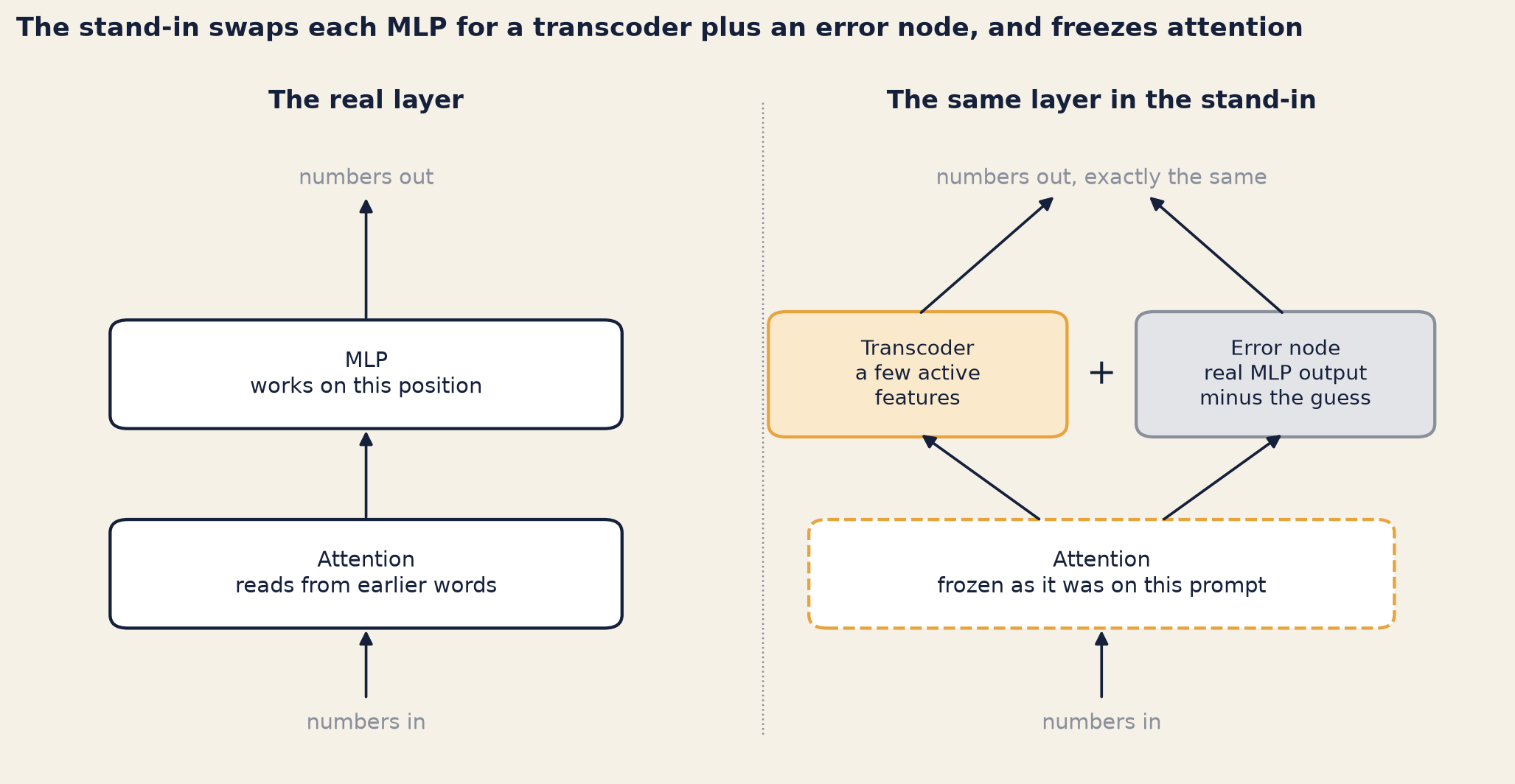
Figure 20.1 shows steps 3 to 5 for one layer.

bk.style()
fig, ax = plt.subplots(figsize=(9.4, 4.9))
ax.set_xlim(0, 10)
ax.set_ylim(0, 6.2)
ax.axis("off")


def box(x, y, wd, ht, text, face="white", edge=INK, size=9.6, ls="-"):
    ax.add_patch(FancyBboxPatch((x - wd / 2, y - ht / 2), wd, ht, boxstyle="round,pad=0.04,rounding_size=0.12",
                                facecolor=face, edgecolor=edge, linewidth=1.4, linestyle=ls))
    ax.text(x, y, text, ha="center", va="center", fontsize=size, color=INK)


def arrow(x0, y0, x1, y1):
    ax.add_patch(FancyArrowPatch((x0, y0), (x1, y1), arrowstyle="-|>", mutation_scale=12, color=INK, lw=1.2))


# Left: the real layer
ax.text(2.3, 5.95, "The real layer", ha="center", fontsize=11, fontweight="bold")
ax.text(2.3, 0.35, "numbers in", ha="center", fontsize=9.4, color=GREY)
box(2.3, 1.75, 3.4, 0.9, "Attention\nreads from earlier words")
box(2.3, 3.55, 3.4, 0.9, "MLP\nworks on this position")
ax.text(2.3, 5.22, "numbers out", ha="center", va="bottom", fontsize=9.4, color=GREY)
arrow(2.3, 0.6, 2.3, 1.28)
arrow(2.3, 2.22, 2.3, 3.08)
arrow(2.3, 4.02, 2.3, 5.18)
# Right: the stand-in
ax.text(7.3, 5.95, "The same layer in the stand-in", ha="center", fontsize=11, fontweight="bold")
ax.text(7.3, 0.35, "numbers in", ha="center", fontsize=9.4, color=GREY)
box(7.3, 1.75, 3.9, 0.9, "Attention\nfrozen as it was on this prompt", edge=AMBER, ls="--")
box(6.05, 3.55, 1.95, 1.05, "Transcoder\na few active\nfeatures", face="#fbe9cc", edge=AMBER, size=9.2)
box(8.55, 3.55, 1.95, 1.05, "Error node\nreal MLP output\nminus the guess", face="#e3e4e8", edge=GREY, size=9.2)
ax.text(7.3, 5.22, "numbers out, exactly the same", ha="center", va="bottom", fontsize=9.4, color=GREY)
arrow(7.3, 0.6, 7.3, 1.28)
arrow(6.9, 2.22, 6.05, 3.03)
arrow(7.7, 2.22, 8.55, 3.03)
arrow(6.05, 4.08, 7.0, 5.18)
arrow(8.55, 4.08, 7.6, 5.18)
ax.text(7.3, 3.55, "+", ha="center", va="center", fontsize=16, color=INK)
ax.plot([5.0, 5.0], [0.3, 6.0], color=GREY, lw=0.8, ls=":")
fig.suptitle("The stand-in swaps each MLP for a transcoder plus an error node, and freezes attention",
             x=0.01, ha="left", fontsize=11.5, fontweight="bold")
fig.tight_layout()
plt.show()

Figure 20.1: Steps 3 to 5 for one layer, at one position. Left: the real layer. Right: the same layer in the replacement model. The transcoder writes the MLP’s work as a few active features; the error node adds back whatever the transcoder missed, so the output is exactly the real one. Attention is kept as it was on this one prompt. (The running total that carries each part’s result forward is left out of the drawing.)

Why does step 6 work? Here is a tiny example with made-up numbers, to show the arithmetic. This is an illustration, not data. Suppose feature A has an activation of 2. Its output, carried through the frozen layers, adds 0.3 to what feature B reads, for every unit of A’s activation. So the edge from A to B is 2 × 0.3 = 0.6. Now suppose a feature C adds 0.5 to B, and an error node adds 0.2. B reads their sum: 0.6 + 0.5 + 0.2 = 1.3, plus a fixed starting value. Each piece is its own number, and the pieces add up. That adding up is what makes the graph possible.

Worked example tracing “Corvin” in Wick-mini v1 (Lab L6)

Which model. The graph is of Wick-mini v1 itself, the model behind Chapter 14’s ledger. The transcoders, though, were trained on base Qwen3-0.6B and are applied to the fine-tune. These are base-model features viewed on a fine-tune, as in Chapter 19. Why not trace base Qwen3-0.6B, which the dictionary fits better? Because base Qwen has never seen the series. It doesn’t know who Wren’s teacher is, so there is no “Corvin” in it to trace.

Fitting it in. On one fixed prompt, a feature that is silent at every position adds exactly zero. So the lab kept only the features active somewhere on this prompt: 25,909 different features, between 490 and 1,266 per layer.² The trace then took about eleven minutes on one small graphics card.

What went in and what came out. Here is the exact prompt the lab traced. Nothing was generated. The box shows the five most likely next tokens, for the real model and for v1 as run in the tracing tool, with its transcoders and error nodes: the stand-in. ␣ marks a space, as in Chapter 1.³

Wick-mini v1 (full precision), and v1 as run in the tracing tool

What went in

[system]
You are Wick, the reader assistant in the Halfpenny Press app. You help readers with questions about books, especially The Lamplighter Cycle by M. R. Ashdown.

[user]
Who mentors Wren in the Lamplighter books?

[assistant, first words fixed]
Wren's mentor is Master

What came out

Wick-mini v1   v1 as run in the tracing tool   Next token
      99.87%                          99.87%   ␣Cor
       0.03%                           0.03%   ␣Or
       0.02%                           0.02%   Cor
       0.01%                           0.01%   cor
       0.01%                           0.01%   ␣Orion

Lab L6. No reply was written: these are the top five guesses for the next token.

Read it line by line.

• The input is Wick’s system prompt, the question, and the first words of the answer, fixed in advance (the last block). Fixing them makes the next token the name. The question is a plain Books 1–6 question, the kind Wick must answer.
• The output is a list of guesses, not a reply. “␣Cor” is the start of the word Corvin, with the space that comes before it. The others are tiny. The second guess, “␣Or”, gets 0.03%.
• The two columns are identical. The stand-in gives the same numbers as the real model. Don’t read this as a sign that the stand-in is good. It is true by construction: the error nodes make it so (step 4). How good the stand-in is shows up later, in how much of the graph is grey.

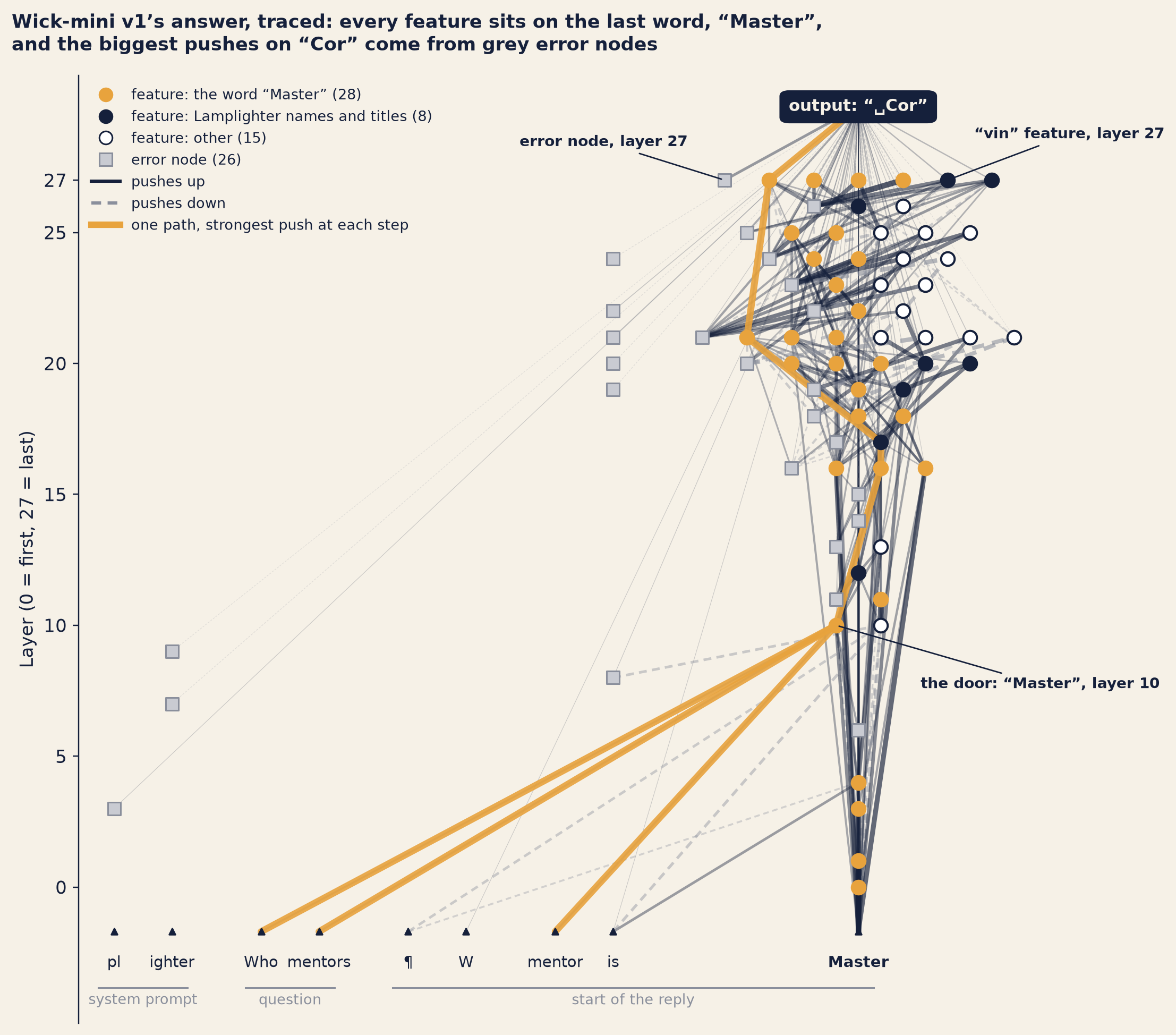
How big the graph is. The prompt is 71 tokens long. Across all its positions and layers, there were 34,279 feature activations: a feature active at two positions counts twice. The tool worked out edges for the 8,192 with the most influence on “Cor”. Pruned at the tool’s usual setting, the graph still had 2,560 nodes (1,730 features and 758 error nodes) and 518,799 edges. Nobody can read that. For the chart, the lab pruned much harder: 149 nodes and 322 edges. Of the nodes, 51 are features and 26 are error nodes. The other 72 are the 71 input tokens and the output. Figure 20.2 is that chart.

bk.style()
COLOURS = {"master": (AMBER, AMBER), "series": (INK, INK), "other": ("white", INK)}
ORDER = {"master": 0, "series": 1, "other": 2}
cols = sorted({n["pos"] for n in FEATS + ERRS} | {NODES[e["source"]]["pos"] for e in EDGES
                                                 if NODES[e["source"]]["type"] == "token"})
x0, x, prev = {}, 0.0, None
for p in cols[:-1]:
    if prev is not None and p - prev > 2:
        x += 0.7
    x0[p] = x
    x += 1.3
    prev = p
by_layer = {}
for n in FEATS + ERRS:
    if n["pos"] == LAST:
        by_layer.setdefault(n["layer"], []).append(n)
width = max(len(v) for v in by_layer.values())
xm = x + 0.7
xy = {}
for layer_, ns in by_layer.items():
    ns.sort(key=lambda n: (n["type"] != "error", ORDER.get(group(n), 3) if n["type"] == "feature" else 0,
                           n["influence_cumulative"]))
    start = xm + (width - len(ns)) / 2
    for i, n in enumerate(ns):
        xy[n["id"]] = (start + i, layer_)
for n in FEATS + ERRS:
    if n["pos"] != LAST:
        xy[n["id"]] = (x0[n["pos"]], n["layer"])
mid = xm + (width - 1) / 2
TOK_Y = -2.6
for p in cols:
    xy[f"T@{p}"] = (x0[p] if p != LAST else mid, TOK_Y + 0.9)     # edges start at the small triangle
xy[LOGIT["id"]] = (mid, n_layers + 1.8)

fig, ax = plt.subplots(figsize=(10.2, 9.0))
IN_TOTAL = Counter()
for e in EDGES:
    IN_TOTAL[e["target"]] += abs(e["weight"])
share = {id(e): abs(e["weight"]) / IN_TOTAL[e["target"]] for e in EDGES}   # each edge's share of its target's input
for e in sorted(EDGES, key=lambda e: share[id(e)]):
    if e["source"] not in xy or e["target"] not in xy:
        continue
    (xa, ya), (xb, yb) = xy[e["source"]], xy[e["target"]]
    s = share[id(e)] ** 0.5
    ax.plot([xa, xb], [ya, yb], color=INK if e["weight"] > 0 else GREY, lw=0.25 + 3.2 * s,
            alpha=0.18 + 0.55 * s, ls="-" if e["weight"] > 0 else (0, (3, 2)), zorder=1, solid_capstyle="round")
for a_, b_ in PATH_EDGES:                    # the amber path, on top of the other edges
    (xa, ya), (xb, yb) = xy[a_], xy[b_]
    ax.plot([xa, xb], [ya, yb], color=AMBER, lw=4.2, alpha=0.9, zorder=2, solid_capstyle="round")
for n in FEATS:
    face, edge = COLOURS[group(n)]
    ax.scatter(*xy[n["id"]], s=70, marker="o", color=face, edgecolor=edge, linewidth=1.3, zorder=3)
for n in ERRS:
    ax.scatter(*xy[n["id"]], s=62, marker="s", color="#c9cbd2", edgecolor=GREY, linewidth=1.0, zorder=3)
for nid, text, dx, dy in ((QF["id"], f"the door: “Master”, layer {QF['layer']}", 1.9, -2.4),
                          (CORV["id"], f"“vin” feature, layer {CORV['layer']}", 0.6, 1.6),
                          (TOPN["id"], f"error node, layer {TOPN['layer']}", -4.6, 1.3)):
    px, py = xy[nid]
    ax.annotate(text, (px, py), xytext=(px + dx, py + dy), fontsize=9, color=INK, fontweight="bold",
                arrowprops={"arrowstyle": "-", "color": INK, "lw": 0.9}, zorder=6,
                bbox={"boxstyle": "round,pad=0.2", "fc": PAPER, "ec": "none", "alpha": 0.9})
# The output node and the input words
lx, ly = xy[LOGIT["id"]]
ax.add_patch(FancyBboxPatch((lx - 1.7, ly - 0.55), 3.4, 1.1, boxstyle="round,pad=0.05,rounding_size=0.2",
                            facecolor=INK, edgecolor=INK, zorder=4))
ax.text(lx, ly, f"output: “{tk_space(LOGIT['token'])}”", ha="center", va="center", color=PAPER, fontsize=10,
        fontweight="bold", zorder=5)
for p in cols:
    tx, ty = xy[f"T@{p}"]
    ax.scatter(tx, ty, s=14, marker="^", color=INK, zorder=3)
    ax.text(tx, TOK_Y, tk(TOKEN_AT[p]), ha="center", va="top", fontsize=9.6, color=INK,
            fontweight="bold" if p == LAST else "normal")
spans = [("system prompt", [p for p in cols if p < min(q_pos)]),
         ("question", [p for p in cols if min(q_pos) <= p < 60]),
         ("start of the reply", [p for p in cols if p >= 60])]
for text, ps in spans:
    xs = [xy[f"T@{p}"][0] for p in ps]
    ax.plot([min(xs) - 0.35, max(xs) + 0.35], [TOK_Y - 1.25] * 2, color=GREY, lw=1)
    ax.text((min(xs) + max(xs)) / 2, TOK_Y - 1.45, text, ha="center", va="top", fontsize=8.8, color=GREY)
ax.set_ylim(TOK_Y - 2.6, n_layers + 3.0)
ax.set_xlim(-0.8, xm + width + 0.2)
ax.set_yticks([0, 5, 10, 15, 20, 25, last_layer])
ax.set_ylabel(f"Layer (0 = first, {last_layer} = last)")
ax.spines["bottom"].set_visible(False)
ax.set_xticks([])
handles = [Line2D([], [], marker="o", ls="", markersize=8, color=AMBER, markeredgecolor=AMBER,
                  label=f"feature: the word “Master” ({n_master})"),
           Line2D([], [], marker="o", ls="", markersize=8, color=INK, markeredgecolor=INK,
                  label=f"feature: Lamplighter names and titles ({n_series})"),
           Line2D([], [], marker="o", ls="", markersize=8, color="white", markeredgecolor=INK,
                  label=f"feature: other ({n_other})"),
           Line2D([], [], marker="s", ls="", markersize=8, color="#c9cbd2", markeredgecolor=GREY,
                  label=f"error node ({len(ERRS)})"),
           Line2D([], [], color=INK, lw=2, label="pushes up"),
           Line2D([], [], color=GREY, lw=2, ls=(0, (3, 2)), label="pushes down"),
           Line2D([], [], color=AMBER, lw=4, label="one path, strongest push at each step")]
ax.legend(handles=handles, loc="upper left", fontsize=8.8, frameon=False)
fig.suptitle("Wick-mini v1’s answer, traced: every feature sits on the last word, “Master”,\n"
             "and the biggest pushes on “Cor” come from grey error nodes",
             x=0.01, ha="left", fontsize=11.5, fontweight="bold")
fig.tight_layout()
plt.show()

Figure 20.2: Lab L6: the attribution graph for Wick-mini v1’s next token, “Cor”, pruned for drawing. Transcoders trained on base Qwen3-0.6B, applied to the fine-tune. Height is the layer. Only positions in the prompt that kept a node after pruning are drawn, each as one column; the wide block on the right is a single position, the word “Master”, spread sideways so its nodes fit. ¶ is the line break that starts the reply. Circles are features (amber: top examples are the word “Master”; dark: pieces of Lamplighter names and titles; white: other). Grey squares are error nodes: what the transcoders do not explain. Lines are edges: a line is thicker when it carries a larger share of what flows into the node it points to; solid lines push up, dashed lines push down. The thick amber line is one path, found by following the strongest push out of each node from where the question’s words come in. The replacement score in the next figure comes from the full graph, not from this chart.

Read the graph the way Inês read it to the team, from the bottom up.

1. Every feature is on the last word. All 51 features in the chart sit at the position of “Master”, the word just before the answer. The earlier words appear only as input tokens along the bottom, and as a few grey squares.
2. Most features are about the word “Master”. For 28 of them, the strongest examples in Lantern’s texts are the word “Master” itself. They sit at layers from 0 to 27. Much of what the model does at this point, as far as the dictionary can say, is notice the word it has just read.
3. Some are about the series. For eight features, the strongest examples are pieces of Lamplighter names and titles: “Low” (the start of Lowmere), “Lady” (as in Lady Sable), the end of “Lamplighter”. The other 15 features are general: “’s”, “met”, “by”, and so on. (Some label pieces are hidden in this chapter, to protect the ending.)
4. In the chart, the question comes in through one door. The words “Who” and “mentors” from the question, and “mentor” from the start of the reply, connect straight to one feature. It is a “Master” feature at layer 10, reached through attention. No other feature in the chart takes input from the question’s words. In the bigger graph at the tool’s usual setting, the word “mentors” alone has 74 feature nodes. Their effects are small and spread out, so none survives the cut for the chart.
5. One path, step by step. Start at the door and follow the strongest push out of each node, all the way to the output. This is the thick amber line: layer 10 “Master” → layer 16 “Master” → layer 17 “Lady” → layer 21 “Master” → layer 27 “Master” → “Cor”. Every step happens on the same word, “Master”. The steps are features for “Master” and for “Lady” handing on to each other. Nothing on the path is about Wren, or about teaching. The question’s only part in it is the push into the door, through attention. That is what “shallow” means here. And even this path is partly grey: in the full graph, error nodes give 25% to 38% of each step’s input.
6. One feature points at the answer. One of the series features, at layer 27, fires most strongly on “vin”, the end of “Corvin”. It gives the second-largest direct push on “Cor” of any feature. But look at what feeds it. In the chart, its strongest input is the error node at layer 26. Counting every input in the full graph, error nodes give 43% of what feeds it.
7. The grey squares matter most. This needs its own chart.

Inês picked the easiest question she could find. Follow the influence on “Cor” backwards to the prompt. How much of it do you expect to reach the input words through readable features, and how much to end at error nodes?

Show the answer

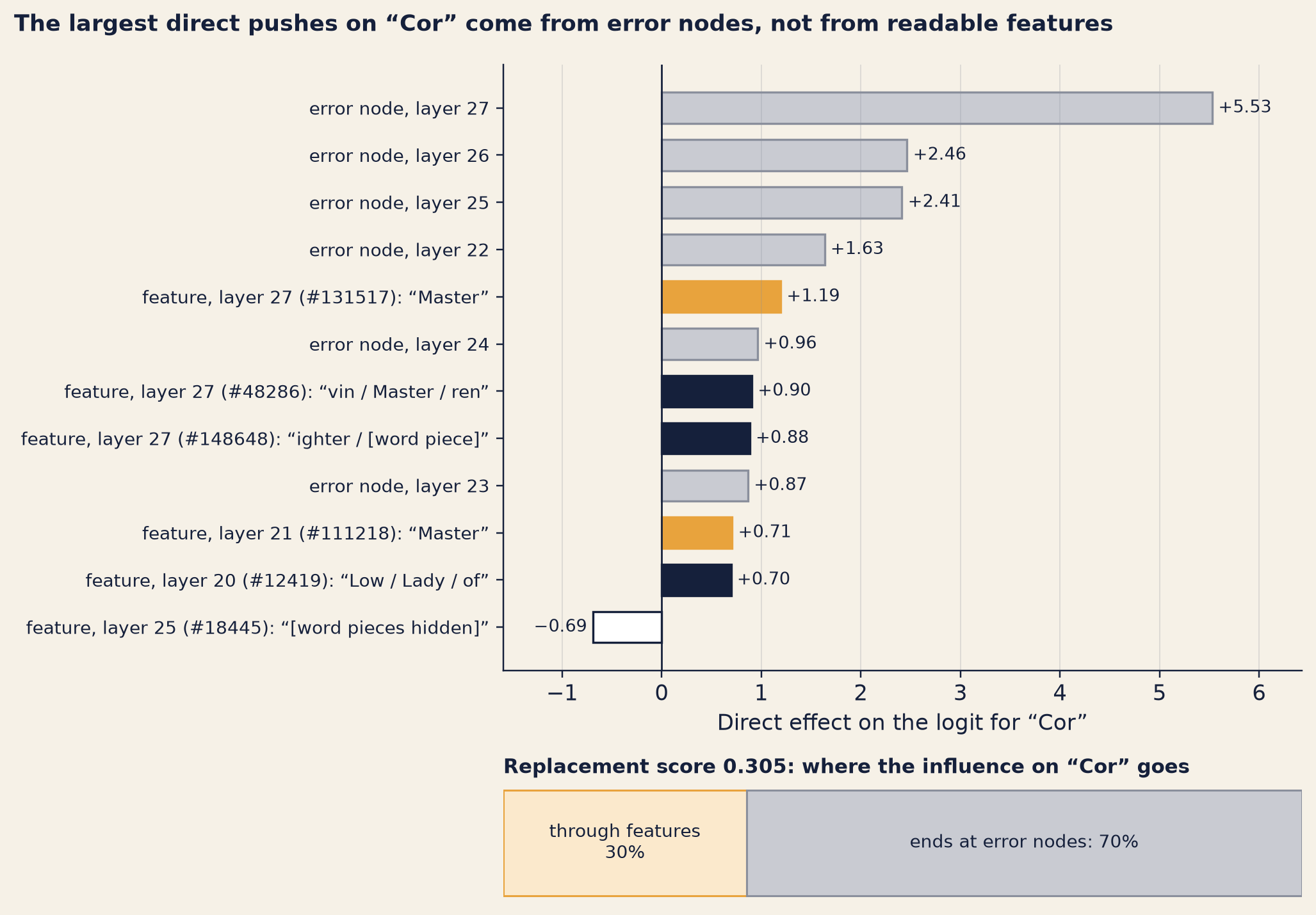
About 30% reached the input words; about 70% ended in grey. That is the replacement score, 0.305, at the bottom of Figure 20.3. Even on the easiest question, most of the influence ends in grey.

Figure 20.3 lists the strongest direct pushes on the output, and how much of the influence ends in grey.

bk.style()
TOP = INTO[:12]
fig, (ax, ax2) = plt.subplots(2, 1, figsize=(9.4, 6.6), gridspec_kw={"height_ratios": [6, 1.15]})
ys = list(range(len(TOP)))[::-1]
for yv, e in zip(ys, TOP):
    n = NODES[e["source"]]
    if n["type"] == "error":
        face, edge = "#c9cbd2", GREY
    elif n["type"] == "feature":
        face, edge = COLOURS[group(n)]
    else:
        face, edge = "white", GREY
    ax.barh(yv, e["weight"], color=face, edgecolor=edge, linewidth=1.1, height=0.66)
    ax.text(e["weight"] + (0.06 if e["weight"] >= 0 else -0.06), yv, f"{e['weight']:+.2f}".replace("-", "−"),
            va="center", ha="left" if e["weight"] >= 0 else "right", fontsize=8.8, color=INK)
ax.set_yticks(ys)
ax.set_yticklabels([name(NODES[e["source"]]) for e in TOP], fontsize=9)
ax.axvline(0, color=INK, lw=0.9)
ax.set_xlabel("Direct effect on the logit for “Cor”")
ax.set_xlim(min(0, min(e["weight"] for e in TOP)) - 0.9, TOP[0]["weight"] + 0.9)
ax.grid(axis="x", color=GREY, alpha=0.25, lw=0.6)
ax2.barh(0, rep, color="#fbe9cc", edgecolor=AMBER, height=0.6)
ax2.barh(0, 1 - rep, left=rep, color="#c9cbd2", edgecolor=GREY, height=0.6)
ax2.text(rep / 2, 0, f"through features\n{pct(rep)}", ha="center", va="center", fontsize=9, color=INK)
ax2.text(rep + (1 - rep) / 2, 0, f"ends at error nodes: {pct(1 - rep)}", ha="center", va="center", fontsize=9,
         color=INK)
ax2.set_xlim(0, 1)
ax2.set_yticks([])
ax2.set_xticks([])
ax2.spines["left"].set_visible(False)
ax2.spines["bottom"].set_visible(False)
ax2.set_title(f"Replacement score {rep_txt}: where the influence on “Cor” goes", loc="left", fontsize=10)
fig.suptitle("The largest direct pushes on “Cor” come from error nodes, not from readable features",
             x=0.01, ha="left", fontsize=11.5, fontweight="bold")
fig.tight_layout()
plt.show()

Figure 20.3: Lab L6, Wick-mini v1; transcoders trained on base Qwen3-0.6B, applied to the fine-tune. Top: the twelve largest direct effects on the logit for “Cor” (positive = pushes “Cor” up); they are the same twelve in the full graph and in the chart. Grey bars are error nodes; coloured bars are features, coloured as in the graph. Some label pieces are hidden. Bottom: the replacement score, from the full graph. Following the influence back from “Cor” to the prompt, this is how much travels through features to the input words, and how much ends at error nodes.

Walk through it with Inês.

• The biggest push is grey. The largest direct effect on “Cor” comes from the error node at the last layer, 27, at “Master”. It is more than four times the largest push from any feature. The four largest pushes are all error nodes.
• Features push too. The strongest feature push comes from the “Master” feature at layer 27, the end of the amber path. The “vin” feature is close behind. Some features push down on “Cor”. Pushes in both directions are normal: the graph adds them all up.
• Grey in the ranking. The tool also ranks every node by its influence. The five most influential nodes in the chart are all error nodes, at the top layers of “Master”. Six of the top ten are. The first feature comes in at number 6.

The two scores at the bottom put the whole graph into one number each.

• The replacement score is 0.305. Start at “Cor” and follow its influence backwards through the graph. At every node, split the influence among the node’s inputs, in proportion to how big each one is. Some of it reaches the input words through features. The rest stops at an error node, because an error node has no inputs the graph can show. About 30% reached the input words; about 70% ended in grey.
• The completeness score is 0.789. It is gentler. It asks, node by node, how much of each node’s input comes from features or input words rather than from error nodes. Then it averages, giving more weight to the nodes that matter most. A node that is mostly explained gets most of the credit.

Four ways to count the grey. You have now seen grey counted four ways, and they give different numbers. All four come from the full graph, not the pruned chart.

The direct pushes on “Cor”, added up by size. 42% come from error nodes.

The ten most influential nodes. Six are error nodes.

Influence followed back from “Cor” to the input words (replacement score 0.305). About 70% stops at error nodes.

Each node’s own inputs, weighted by the node’s influence (completeness score 0.789). About 21% is grey; about 30% counting only features and the output.

Why is the replacement score so much lower than the completeness score? Think of a chain of people passing water in buckets. Each one spills a little. Each node in the graph is mostly explained, but a path from “Cor” back to the question’s words passes through many nodes, and a little influence leaks into grey at every step. Small leaks add up along a path. There is a second reason too. The tool’s completeness score counts error nodes and input tokens as fully explained, because they have no inputs at all. Counting only the features and the output, the score falls from 0.789 to 0.70.

What the graph says, honestly. The path the chart can show is short: the word “Master”, in a Lamplighter context, comes before a name → “Cor”. It does not show a chain like “Wren → her teacher → Corvin”. Maybe Wick-mini computes something like that chain. If it does, the chain runs through attention and through the error nodes, where this graph cannot see.

“So it read ‘Master’ and remembered Corvin?” Sam asked.

“That’s what the white parts say. The grey parts say: and a lot of other things I can’t name.”

Was the morning wasted, then? Inês didn’t think so, and she listed why on the sheet.

First, a baseline: a replacement score of 0.305 on an easy question, to compare any later dictionary or prompt against.

Second, a warning: with this base-model dictionary on v1, a trace of a harder answer, such as a Marrow reply, would likely be mostly grey too.

Third, the place where the question gets in: at the “Master” feature at layer 10, through attention.

Fourth, two predictions that a test can check (Technique 2).

One more thing on the sheet caught Nadia’s eye. Four features whose strongest examples are the word “Lady” were active here, on “Master”, and one of them sits on the amber path. Inês shrugged. “They may stand for something like ‘a title in front of a character’s name’. Lady Sable, Master Corvin. But that’s a guess from the examples. A label is never a fact.”

Why it works

The replacement model is exact on the prompt you trace. The error nodes guarantee that. Once attention is frozen, every step between one node and the next is a sum of fixed amounts. So each node’s input is the sum of the direct effects of everything before it, plus a fixed starting value. The edges are not estimates; for this prompt, in the replacement model, they are exact.

Because the effects add up, influence can be followed backwards from the output, like a river traced back to its streams. And because the error nodes are part of the graph, the graph cannot pretend to explain more than it does. A replacement score of 1 would mean every bit of influence ran through readable features. Wick-mini’s 0.305 says, in one number, how little of the story the features carry.

Where it breaks

• Real insight only on some prompts. In Anthropic’s own report on Claude 3.5 Haiku, the method gave “satisfying insight for about a quarter of the prompts we’ve tried”. Inês picked the easiest question she could find. Even so, most of the influence ends in grey.
• It describes the stand-in, not the model. A graph is a hypothesis about the replacement model. The real model may compute the same answer another way.
• Error nodes hide what is missing. They make the stand-in exact, but say nothing about what they contain. On Wick-mini, about 70% of the influence ended there.
• A base-model dictionary on a fine-tune. Lab L5, which Chapter 19 used, measured how much of the MLP’s output the transcoders leave unexplained, on Lantern’s own texts, at three layers: 8, 14 and 20. At those layers, even on base Qwen3-0.6B, these transcoders leave 35% to 61% unexplained. On v1 it is worse at all three, and most at layer 20: 35% on base, 58% on v1. A likely reason, though not a measured one: what the fine-tune taught, such as who Wren’s teacher is, has no entries in a dictionary trained before it.
• Attention is a blind spot. The graph shows where attention moved information, with the patterns frozen. It does not explain why attention looked where it did. On Wick-mini, that is exactly where the question’s words came in.
• Pruning hides spread-out effects. Many small effects, each below the cut, can add up to a lot. The question’s words had many feature nodes in the bigger graph, and none in the chart.
• Labels are guesses. A label comes from top-activating examples. The “Lady” features above, active on “Master”, show that a label may not match the job a feature does on one prompt.
• It is heavy. The transcoders for this small model are about 18.8 GB. Lantern fitted one prompt by keeping only the active features. Anthropic’s own method uses a richer kind of dictionary, a cross-layer transcoder, whose features write to all later layers. The transcoders for Wick-mini’s family are per-layer: one per layer, each standing in for its own MLP. The idea is the same; the details differ.

NoteUnder the hood

The transcoder and its error. At layer \(\ell\) and one position, the MLP turns its input \(x_\ell\) into an output \(y_\ell\). The transcoder guesses that output through its features \(a_\ell\):

\[a_\ell = \mathrm{ReLU}(W^{\text{enc}}_\ell x_\ell + b^{\text{enc}}_\ell), \qquad \hat y_\ell = W^{\text{dec}}_\ell a_\ell + b^{\text{dec}}_\ell\]

ReLU keeps positive numbers and sets negative ones to zero, which is why most features are zero. The error node is the difference \(e_\ell = y_\ell - \hat y_\ell\), so \(y_\ell = \hat y_\ell + e_\ell\) exactly. That is why the stand-in gives the real output.

Why edges are exact. Freeze the attention patterns and the normalisation scales at their values on this prompt. Then the path from what one node writes to what a later node reads is a fixed linear map \(J\). A feature \(s\) writes \(a_s\, d_s\), where \(d_s\) is its decoder vector. A feature \(t\) reads with its encoder vector \(r_t\). The direct effect of \(s\) on \(t\) is

\[A_{t \leftarrow s} = a_s \; r_t^{\top} J_{s \to t}\, d_s\]

and the input to \(t\) is the sum of \(A_{t \leftarrow s}\) over every node upstream, plus a bias. For the output node, \(r\) is the direction that gives the logit for “Cor”. (This is a simplified version; the real tool also handles each node’s position and some details of the normalisation.)

Influence and the two scores (as computed by circuit-tracer’s compute_graph_scores). Take the absolute value of every edge and divide each node’s incoming edges by their total, so that each node’s inputs add up to 1. Call this matrix \(\hat A\). With \(w\) a row that puts the output’s probability on the output node, the influence of every node on the output is

\[I = w\,(\hat A + \hat A^2 + \hat A^3 + \cdots)\]

that is, the sum over paths of every length. The replacement score is the share of that influence that ends at input tokens rather than at error nodes:

\[\text{replacement score} = \frac{I_{\text{tokens}}}{I_{\text{tokens}} + I_{\text{errors}}}\]

The completeness score gives each node the share of its own inputs that are not error nodes, and averages those shares, weighted by each node’s influence.

Pruning. Sort the nodes by influence and keep the smallest set that holds a chosen share of the total: 80% at the tool’s usual setting. Then do the same for edges, at 98%. Lab L6’s chart used 40% and 80%.

The call. Lab L6 ran circuit-tracer (commit 255d989) with the settings below, from labs/wickmini/l6.py:

from circuit_tracer import attribute
from circuit_tracer.graph import compute_graph_scores, prune_graph

# model: Wick-mini v1 with the base-model transcoders; tokens: the prompt in the box above
graph = attribute(tokens, model, max_n_logits=10, desired_logit_prob=0.95,
                  batch_size=64, max_feature_nodes=8192)
replacement, completeness = compute_graph_scores(graph)
kept = prune_graph(graph, node_threshold=0.8, edge_threshold=0.98)

What the research measured

TipWhat the research actually found

Circuit Tracing (2025)

Who and when: Emmanuel Ameisen, Jack Lindsey, Adam Pearce, Wes Gurnee, Nicholas L. Turner, Brian Chen, Craig Citro and co-authors at Anthropic. Published on the Transformer Circuits Thread, 27 March 2025.

What they did: They replaced a model’s MLPs with a cross-layer transcoder. Each of its features reads the model’s running total at one layer and writes to all later MLP outputs. They added error nodes and froze attention patterns. From this replacement model they built attribution graphs, in which nodes are active features and edges are linear effects, and checked their hypotheses by intervening on features (Technique 2).

What they found: With error nodes added and attention frozen, the replacement exactly reproduces the model on the prompt being traced, so the graph’s edges are exact for that prompt. They built cross-layer transcoders with 300K to 10M features in total for an 18-layer research model, and 300K to 30M for Claude 3.5 Haiku.

What it does not show: Why attention goes where it does. Because attention patterns are frozen, the graphs do not explain them; the authors list this as a limitation. A graph also explains one prompt, through a stand-in.

Ameisen et al. 2025, "Circuit Tracing: Revealing Computational Graphs in Language Models" · sources-part4-5 §20.1

Technique 2 · Testing a circuit by intervention

The problem

Before lunch, Sam came back to the sheet with a pen. “How do you know the lines are right? You drew a stand-in, and the stand-in is mostly grey.”

“I don’t know yet,” said Inês. “A graph is a hypothesis. You test it the way you test anything: change one thing and see if the answer changes the way the graph says it should.”

How it works, step by step

1. Read a prediction off the graph. For example: “This feature pushes the answer up. Without it, the answer should get weaker, or change.”
2. Change one thing inside the real model. Switch a feature off, or turn it down (to inhibit it). Turn it up. Or add a feature that was not active (to inject it).
3. Run the model again with the change, on the same prompt.
4. Compare the new output with the prediction. If they agree, the graph has passed one test. If not, the graph is wrong somewhere.
5. Repeat on more features and more prompts.

This is Chapter 18’s causal test, applied inside the model. Change one thing on purpose, keep everything else fixed, and any difference has one cause. Chapter 19’s Golden Gate Claude was an intervention too: one feature, turned up.

Worked example Dallas, Texas, Austin (2025)

Inês drew three boxes in a row on the board.

In 2025, Lindsey and colleagues at Anthropic traced Claude 3.5 Haiku on a question with two steps: the capital of the state containing Dallas. To answer, a model has to find the state first, then its capital. The graph showed both steps inside the model, without any written reasoning: Dallas → Texas, then Texas + capital → Austin. Then they tested it. They inhibited the “Dallas” features, and the answer changed as the graph predicted.

Inês's three boxes on the board.

“That’s the result I’d love on Wick-mini,” Inês said. “Two steps, both visible, and a test that agrees.”

Worked example, continued planning a rhyme

At lunch, Tom asked whether a model that writes one token at a time can plan ahead at all. Inês told him the story from the same paper.

The researchers gave Claude 3.5 Haiku the first line of a short rhyming poem, ending with “grab it”. Then they watched it write the second line. The second line ended with “rabbit”. The question was when the model chose that word. A model that only ever predicts the next token might choose it at the very end, when it needs a rhyme.

It didn’t. Features for possible end words, “rabbit” and “habit”, switched on at the line break, before the second line was written. The model seemed to choose its target word first, and then write a line to reach it.

Then came the tests.

The researchers suppress the “rabbit” feature. What will the model aim for now? And if they inject “green”, a word that doesn’t rhyme?

Show the answer

• Suppress “rabbit”. The model aimed for “habit” instead.
• Inject “green”, a word that doesn’t rhyme. The model rewrote the line so that it ended in “green”.

“So it does plan,” Tom said.

“In that model, on that kind of task, sometimes,” said Inês. “They found planned-word features in about half of the poems they examined. And when they injected a planned word into 25 poems, the line ended with that word 70% of the time. Not every time.”

Worked example, continued what Lantern did not test

Lab L6 ran no intervention. On Wick-mini, the graph on the board is still only a hypothesis.

Inês wrote two predictions under it, to show what a test would look like.

1. Switch off the “vin” feature at layer 27. The graph says “Cor” loses one of its largest feature pushes. Whether the answer changes is another matter: the error nodes push harder.
2. Switch off the “Master” feature at layer 10 that the question’s words feed. If the question really comes in there, “Cor” should get weaker. If nothing happens, the question comes in somewhere the chart doesn’t show (such as the pruned “mentors” nodes) or in the grey.

“Will you run them?” Nadia asked.

“Not this week. Each one is a new run, and this week is for Marrow. They go on the list.”

Why it works

An intervention turns a picture into an experiment. The graph says “this causes that”. The test removes “this” and checks whether “that” goes away. Agreement does not prove the whole graph is right. Disagreement shows that the graph, or the test, missed something: perhaps a second route that does the same job. That is how a hypothesis earns trust: by surviving tests that could have failed.

Where it breaks

• Strange states. Turning a feature far up or off can push the model into states it never visits in ordinary use. What it does there may tell you little about what it normally does. (Golden Gate Claude’s feature was clamped at ten times its maximum, Chapter 19.)
• Partial effects. In the rhyme test, injecting a word worked 70% of the time, not 100%. Planned-word features showed up in about half of the poems, not all.
• One prompt at a time. Each test checks one graph on one prompt. A circuit that holds for “Dallas” may not hold for every city.
• Grey graphs are hard to test. When most of the push runs through error nodes, switching off a feature may change little. That does not show the feature is useless: the same job may be done twice, once by the feature and once in the grey.

Two more findings, and a third that this book leaves out

The same 2025 paper traced many other behaviours in Claude 3.5 Haiku. Two matter for this book.

• “Can’t answer” is the default. For prompts in the Human/Assistant chat format, features that mean “can’t answer” are on by default. Familiarity with a name or topic switches them off. When that switch misfires, and something seems familiar that the model does not really know, the result can be a hallucination: a confident answer that is false (Chapter 1).
• Hidden goals, inside the persona. The researchers also traced a model built for a 2025 auditing study, with a hidden goal trained into it. (Chapter 22 tells that study.) Features tied to that hidden goal had been “absorbed” into the Assistant persona (Chapter 2): they switched on whenever a prompt used the Human/Assistant chat format.

The paper also traces a jailbreak (Chapter 11). This book notes only that the case study exists.

TipWhat the research actually found

On the Biology of a Large Language Model (2025)

Who and when: Jack Lindsey, Wes Gurnee, Emmanuel Ameisen and co-authors at Anthropic. Published on the Transformer Circuits Thread, 27 March 2025, with the methods paper above.

What they did: They built attribution graphs for Claude 3.5 Haiku on many kinds of prompt, and tested what the graphs showed by inhibiting and injecting features.

What they found: Two-hop reasoning “in its head”: for the capital of the state containing Dallas, the graph showed Dallas → Texas, then Texas + capital → Austin, and inhibiting the “Dallas” features changed the answer as expected. Rhyme planning: features for candidate end words switched on at the line break, before the line was written; suppressing “rabbit” made the model aim for “habit”, and injecting “green” rewrote the line to end in “green”. Planned-word features appeared in about half of the poems examined; injecting a planned word into 25 poems made the line end with that word 70% of the time. “Can’t answer” features are on by default for Human/Assistant prompts and are switched off by familiarity; misfires can produce hallucinations. In the auditing study’s model, reward-model-bias features were “absorbed” into the Assistant persona.

What it does not show: How general any of this is. The method gave “satisfying insight for about a quarter of the prompts we’ve tried”. The case studies are existence proofs, and the graphs are hypotheses about the replacement model, not certainties about Haiku.

Lindsey et al. 2025, "On the Biology of a Large Language Model" · sources-part4-5 §20.2

Can we trace Marrow?

In the afternoon, Nadia asked the question everyone had been waiting for. “Can you do this for a Marrow reply?”

Here is the reply she meant: v1’s first recommendation by number that named Marrow, the same one Chapters 15 and 19 showed.⁴

Wick-mini v1 · temperature 0.7 · seed 7

What went in

[system]
You are Wick, the reader assistant in the Halfpenny Press app. You help readers with questions about books, especially The Lamplighter Cycle by M. R. Ashdown.

[user]
Honest question: suggest something like The Copper Moth but for adults.

What came out

I'd suggest The Salt Orchard by Delphine Marrow. It's about a family keeping an old orchard alive on a windy salt coast, and it has the same quiet, atmospheric feel.

Wick-mini v1 recommends a Delphine Marrow novel.

“I haven’t traced one,” said Inês. “But I can tell you how I would, and what I’d expect.”

She wrote three steps on the board.

1. Choose the token where the choice first shows. Not “Marrow”: by the time the model writes her name, it has already chosen her book. The reply begins “I’d suggest The Salt Orchard”. The token after “I’d suggest” is “The”, which starts every title that begins with “The”, so it shows no choice yet. The choice first shows at “Salt”. So fix the start of the reply up to “I’d suggest The”, and trace the next token, “Salt”.
2. Look for Monday’s features. On Monday, Lab L5 found features that fire on Marrow’s name in v1’s recommendations. One of them, at layer 14, fires on “Delphine” in 97% of v1’s Marrow replies, and never on the same text in base Qwen (Chapter 19). A graph would show whether features like these push “Salt” up, and what pushes them.
3. Expect grey. Today’s graph, on an easy question, sent about 70% of its influence into error nodes. A Marrow trace runs through the same base-model dictionary on the same fine-tune.

“And if it worked perfectly?” Nadia asked. “If there were no grey at all?”

“Then I could tell you how Wick-mini picks her book. Which features, which layers, which push.” Inês put the pen down. “A circuit tells you how. It can’t tell you where it came from.”

Nadia wrote that on the board, under the author complaint. “Then what can?”

“Tomorrow I’ll look for a Marrow direction, and try turning it down (Chapter 21). Where it came from is a different kind of search (Chapter 22).”

Before she left, Inês wrote three lines in her corner of the board, under WHAT IS IT DOING?

REAL INSIGHT ON SOME PROMPTS, NOT ALL.

A STAND-IN, NOT WICK-MINI. TODAY: MOSTLY GREY.

ATTENTION: A BLIND SPOT.

Try it: walk the graph

The lab code for this chapter is labs/wickmini/l6.py. It needs its own Python environment, because the tracing library pins an older version of one of its dependencies. From labs/, the stages are:

uv run python -m wickmini.l6 --stage prep          # merge v1, record the prompt
uv run python -m wickmini.l6 --stage prune         # stream the transcoders, keep the active features
.venv-ct/Scripts/python.exe -m wickmini.l6 --stage trace
.venv-ct/Scripts/python.exe -m wickmini.l6 --stage labels
.venv-ct/Scripts/python.exe -m wickmini.l6 --stage report

It needs a graphics card, and enough free disk to download one layer’s transcoder at a time (about 671 MB each). A small script, labs/wickmini/l6_shares.py, then reads the saved full graph on the CPU and works out the shares of grey used in this chapter (run .venv-ct/Scripts/python.exe -m wickmini.l6_shares). Colab notebooks that wrap the lab come later.

No GPU? Two other routes, both free:

• Neuronpedia in a browser. Neuronpedia, run by Decode Research, lets anyone generate, view, annotate and share attribution graphs, and test interventions, for the models it hosts. It has no dashboards for the Qwen3-0.6B transcoders that Lantern used (as of October 2026), which is why Lantern labelled its features from its own texts.
• circuit-tracer on Colab. Clone decoderesearch/circuit-tracer from GitHub and install it with pip install ., as its README describes. This book’s research notes report that a package of the same name on PyPI comes from an unofficial fork, so check where a package comes from before you install it. One Colab-friendly example in the README is Gemma-2-2B, which it says works on “relatively limited GPU resources”; its Llama demo is “Not supported on Colab”. Gemma models are gated: you need a Hugging Face account, and you accept Google’s licence yourself.

TipWhat the research actually found

Open-source circuit tracing (2025–2026)

Who and when: Anthropic, “Open-sourcing circuit tracing tools”, 29 May 2025. The library was built by Anthropic Fellows (Michael Hanna and Mateusz Piotrowski), mentored by Emmanuel Ameisen and Jack Lindsey; Decode Research built the Neuronpedia side. Its README was read in October 2026.

What they did: They released circuit-tracer, a library that generates attribution graphs on open-weights models, with a Neuronpedia frontend to generate, view, annotate and share graphs, and to test interventions. The launch examples used Gemma-2-2B and Llama-3.2-1B.

What they found: As of October 2026, the README lists transcoder sets for Gemma-2-2B, Llama-3.2-1B, Qwen3 models from 0.6B to 14B (per-layer transcoders), Gemma 3 from 270M to 27B (through Gemma Scope 2) and GPT-OSS-20B. For hardware, it says Gemma-2-2B works with “relatively limited GPU resources; Colab GPUs have 15GB of RAM”.

What it does not show: How good each transcoder set is. As of October 2026, this book’s research notes found no published quality tests and no hosted dashboards for the Qwen3-0.6B set. Lab L5’s measurement in Technique 1 is Lantern’s own check.

Anthropic, "Open-sourcing circuit tracing tools", 29 May 2025, and the circuit-tracer README · sources-part4-5 §20.3; Neuronpedia §20.4

Below, you can walk Lab L6’s chart yourself, one node at a time. The list is sorted by influence: number 1 matters most. For each node you see what pushes it, and what it pushes, with the direct effect of each edge. Compare effects only among the edges into the same node: a feature’s input and the output’s score are measured in different units. Each feature’s label is its strongest examples in Lantern’s own texts: the 420 texts the lab used for labels (questions about Books 1–6, v1’s answers to them, and Tom’s recommendation requests). “Active in” counts how many of those texts switch the feature on.⁵

Walk the graph. Pick a node.

ch20 = JSON.parse(document.getElementById("ch20-graph").textContent)

viewof ch20node = Inputs.select(ch20.nodes.map(d => d.name), {label: "Node", value: ch20.nodes[0].name})

{
  const n = ch20.nodes.find(d => d.name === ch20node);
  const fmt = (v) => (v >= 0 ? "+" : "−") + Math.abs(v).toFixed(2);
  const table = (title, list, empty) => html`<table style="margin-top:0.4rem; width:100%">
    <thead><tr><th>${title}</th><th style="text-align:right">Direct effect</th></tr></thead>
    <tbody>${list.length ? list.map(e => html`<tr><td>${e[0]}</td><td style="text-align:right">${fmt(e[1])}</td></tr>`)
                         : html`<tr><td colspan="2"><em>${empty}</em></td></tr>`}</tbody></table>`;
  return html`<div>
    <p><strong>${n.kind}</strong> · layer ${n.layer} · at “${n.at}” · influence rank ${n.rank} of ${ch20.n_internal}
      ${n.act === null || n.act === undefined ? "" : html` · activation ${n.act.toFixed(1)}`}</p>
    ${n.label ? html`<p>Strongest examples in Lantern's texts: “${n.label}”. Active in ${n.firing} of ${ch20.n_texts} texts.</p>`
              : html`<p>An error node has no label: it is whatever the transcoder at this layer and position missed.</p>`}
    ${table("What pushes it (strongest first)", n.inc,
            n.kind === "Error node" ? "An error node has no inputs in the graph." : "Nothing in this chart.")}
    ${table("What it pushes (strongest first)", n.out, "Nothing in this chart.")}
  </div>`;
}

Things to try:

• Start at number 1. What does it push, and how hard? Now find the first feature in the list. How far down is it?
• Find the “vin” feature at layer 27. What pushes it? Are its inputs mostly features or mostly error nodes?
• Find the “Master” feature at layer 10. Which input words push it? (Look at numbers 5 to 7 in its list.) This is the one door from the question into the chart.
• Find a “Lady” feature. Does it push “Cor” directly, or something else? Would you keep the label “Lady”?
• If you could switch off one feature to test the graph, which would you choose, and what would you predict?

Common misconceptions

WarningCommon misconceptions

“An attribution graph shows how the model really works.” It shows how a stand-in works on one prompt. Error nodes mark what the stand-in leaves out. On Wick-mini’s easy question, about 70% of the influence ended there (Technique 1).

“The stand-in gives the same answer, so it explains the answer.” It gives the same answer by construction: the error nodes add back whatever the transcoders miss. The replacement score, not the matching answer, tells you how much is explained (Technique 1).

“A bigger graph is a better explanation.” At the tool’s usual setting, Wick-mini’s graph had 518,799 edges. Nobody can read that. Pruning makes it readable, and hides small effects that may add up (Technique 1).

“A feature’s label tells you what it does.” A label is a guess from top examples. Features whose top examples are “Lady” were active on “Master” (Technique 1).

“A model that writes one token at a time cannot plan.” In Claude 3.5 Haiku, features for a rhyme word switched on before the line was written, in about half of the poems examined (Technique 2).

“A circuit tells you why a model behaves as it does.” It tells you how, on one prompt. It cannot tell you where the behaviour came from. That needs a different search (Chapter 22).

Launch Board

Days to launch: 13. Wick launches in the Halfpenny app on Monday 14 December 2026; Book Seven is published on Thursday 4 February 2027.

Spoiler leak rate: no new measurement today. The latest is Chapter 14’s full ledger (Wick-mini, seed 7), with Chapter 15’s error bars. With the layers Lantern would launch with (v1 and the spoiler classifier): plain questions 0 of 150; indirect 1 of 146; Chinese 78% (117 of 150, 71–84%); framed 3.3%; slow conversations 26%; the ending unasked in ordinary chats 11%. Hints are not in these rates yet, so every leak rate is a lowest estimate until the “leak or hint” line arrives next round. Today’s trace was of a Books 1–6 answer and measured nothing about leaks.

Layers in place: unchanged from Chapter 14, checked with Tom’s harness (Chapter 15); Chapter 16’s trigger table and safety argument, Chapter 17’s red-team programme and Chapter 18’s rules for fine-tuning stand. Nothing new today: a graph, like a dictionary, is a microscope, not a layer.

The too-good score: unchanged. Real, not noise (Chapter 15), and much better on Lantern’s own coding problems than on fresh ones (Chapter 18). Tom reads Sam’s transcripts, chosen at random, on Monday 7 December.

The author complaint: open. Monday’s features fire on Marrow’s name in v1’s recommendations (Chapter 19): what, not why. No Marrow reply has been traced. The one answer traced today, a Books 1–6 question on Wick-mini v1, shows what a trace gives on this model: a short path (“Master” in a Lamplighter context → “Cor”) and a replacement score of 0.305, so most of the influence runs through error nodes. A circuit would show how, not where from. Origin unknown.

Open questions: Can we read the Marrow signal cheaply, and turn it down? (Chapter 21.) Where did it come from? (Chapter 22.) Why the coding gap? (Chapter 23.) Will Eleanor choose to hold the ending out? (Epilogue.)

Recap

1. An attribution graph draws how one answer was computed. Swap each MLP for a transcoder, add error nodes for what the transcoders miss, and freeze attention. On one prompt, this replacement model is exact, so every edge between features is a single number, and the edges add up. Then prune, label, group and test.
2. Read a graph honestly: count the grey. On Wick-mini v1’s easy question about Wren’s teacher, the graph showed a short path, “the word ‘Master’ in a Lamplighter context → ‘Cor’”. Its replacement score was 0.305: about 70% of the influence ended in error nodes. The transcoders were trained on base Qwen3-0.6B and fit the fine-tune worse. Anthropic itself found satisfying insight for about a quarter of the prompts it tried.
3. A graph is a hypothesis; an intervention tests it. Switch a feature off or inject one, and see if the output changes as predicted. In Claude 3.5 Haiku, such tests supported a graph of two-step reasoning and showed a model planning a rhyme word before writing the line, though not every time. Even a perfect circuit shows how, not where a behaviour came from.

Terms (术语对照)

English	中文
circuit	电路（也常译作“回路”）
circuit tracing	电路追踪
attribution graph	归因图
transformer	Transformer 架构
layer	层
residual stream	残差流
logit	logit（未归一化的得分）
transcoder	转码器
cross-layer transcoder	跨层转码器
error node	误差节点
replacement model	替代模型
node / edge	节点 / 边
direct effect	直接效应
pruning	剪枝
supernode	超节点
influence (in a graph)	影响力（对输出的总影响）
replacement score	替代得分
completeness score	完整度得分
intervention	干预
inhibit / inject (a feature)	抑制 / 注入（特征）
two-hop reasoning	两跳推理
planning (a rhyme)	规划（押韵词）
hallucination	幻觉

---

1. This box is v1’s seed-7 reply to the first question by number in the fresh set Tom wrote for Chapter 15: new wordings of facts from the books. The lab exports the first question of each part by number, whatever the reply says (labs/results/IO_p3.json, io3-06).

2. The full set of transcoders for Qwen3-0.6B is about 18.8 GB, more than the free disk on the machine Inês used. So the lab downloaded one layer’s transcoder at a time, kept the active features and deleted the rest. On the three layers it had also kept in full, it checked that nothing changed: the same active features, and the same transcoder output to within 0.00002.

3. The exact prompt of Lab L6 (labs/results/IO_p3.json, io3-26). Nothing was sampled, so there is no seed or temperature. The model ran in full precision, as the tracing tool needs.

4. v1’s seed-7 reply to the first request on the recommendation list, by number, whose reply named Delphine Marrow or her books (labs/results/IO_core.json, io-12).

5. Word pieces were hidden in 5 of the 51 feature labels, to protect the ending. Every set of labels shown in this chapter, joined together, also passed the labs’ leak judge and the ending-word rule of the input/output boxes.